22 Supplementary Figure 17

22.1 Summary

This is the accessory documentation of Supplementary Figure 17.

The Figure can be recreated by running the R script S17.R:

cd $WORK/3_figures/F_scripts

Rscript --vanilla S17.R
rm Rplots.pdf

22.2 Details of S17.R

In S17.R script is the F3.R script run including additional data sets. Is an executable R script that depends on a variety of image manipulation and data managing and genomic data packages.

It depends on the same helper script as F3.R (F3.functions.R). Additionally it depends on S17.plot_fun.R (modified F3.plot_fun.R) which itself depends on F3.getDXY.R, F3.getFSTs.R,S17.getGxP.R,S17.getIHH12.R, S17.getPIpw.R, S17.getPI.R and S17.getXPEHH.R (all located under $WORK/0_data/0_scripts).

For a detailed documentation please refer to F3.R. The only differences between the two scripts are located in S17.plot_fun.R (compared to F3.plot_fun.R).

22.2.1 Additions in S17.plot_fun.R

In the following additions to S17.plot_fun.R are shown which are missing in the original.

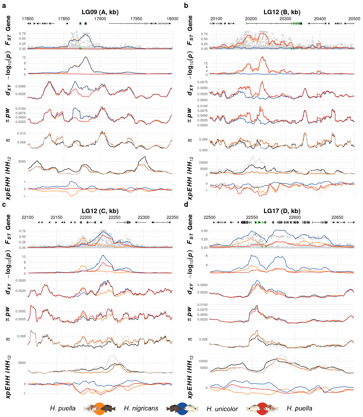
In the beginning, four new helper scripts are loaded which include the data import for the additional parameter which are plotted in Supplementary Figure 15 (\(\pi\), pairwise \(\pi\), iHH₁₂ and xpEHH).

#....#
  source('../../0_data/0_scripts/S17.getGxP.R')
  source('../../0_data/0_scripts/S17.getPI.R')
  source('../../0_data/0_scripts/S17.getPIpw.R')
  source('../../0_data/0_scripts/S17.getIHH12.R')
  source('../../0_data/0_scripts/S17.getXPEHH.R')
#....#

The imported data are stored in data_* vectors.

#....#

  # get pfst values
  pfst_list <- getGxP(searchLG,xr)
  #  data_pfst_pw<-pfst_list$data_pfst_pw;
  data_pfst<-pfst_list$data_pfst

  # get pi values
  piPW_list <- getPIpw(searchLG,xr)
  data_piPW<-piPW_list$data_piPW

  #....#

  # get xpEHH values
  xpEHH_list <- getXPEHH(searchLG,xr)
  data_xpEHH<-xpEHH_list$data_xpEHH
#....#

For each new parameter, an additional plot is created.

    #....#
  p13 <-  ggplot()+coord_cartesian(xlim=xr)+
    geom_line(data=(data_pfst %>% filter(POS > xr[1],POS<xr[2]))
              ,aes(x=POS,y=avgp_wald,col=run),lwd=LW)+
    #....#
    
  p15 <-  ggplot()+coord_cartesian(xlim=xr)+
    geom_line(data=(data_piPW %>% filter(POS > xr[1],POS<xr[2]))
              ,aes(x=POS,y=PI,col=run),lwd=LW)+
    #....#

  p18 <-  ggplot()+coord_cartesian(xlim=xr)+
    geom_line(data=(data_xpEHH %>% filter(POS > xr[1],POS<xr[2]))
              ,aes(x=POS,y=AVGxxEHH,col=run),lwd=LW)+
    #....#
#....#

The plot composition returned by the function includes the additional new plots:

  #....#
  p2 <- plot_grid(p11,p12,p13,p14,p15,p16,p17,p18,
                  ncol = 1,align = 'v',axis = 'r',rel_heights = c(.85,rep(1,6)))
  return(p2)

Comparing to the original script (F3.plot_fun.R):

  #....#
  p2 <- plot_grid(p11,p12,p13,p14,
                  ncol = 1,align = 'v',axis = 'r',rel_heights = c(1.3,rep(1,3)))
  return(p2)

---