19 Supplementary Figure 14

19.1 Summary

This is the accessory documentation of Supplementary Figure 14.

The Figure can be recreated by running the R script S14.R:

cd $WORK/3_figures/F_scripts

Rscript --vanilla S14.R
rm Rplots.pdf

19.2 Details of S14.R

In the following, the individual steps of the R script are documented. Is an executable R script that depends on a variety of image manipulation, data managing and genomic data packages.

It Furthermore depends on the R scripts S09.functions.R (located under $WORK/0_data/0_scripts).

library(tidyverse)
library(scales)
library(cowplot)
library(grid)
library(gridSVG)
library(grImport2)
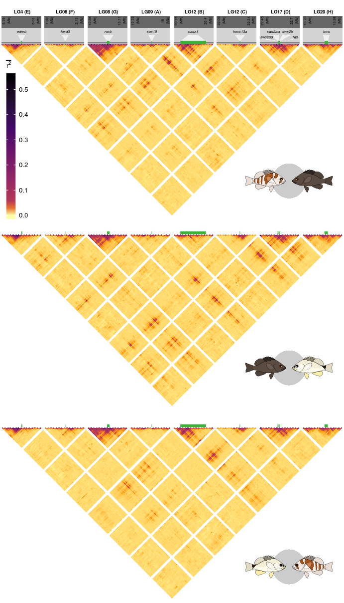
source('../../0_data/0_scripts/S11.functions.R')

The script S09.functions.R contains a function (trplot()) that plots a single LD triangle as seen in Supplementary Figure 14.

The Details of this script are explained in the documentation of F4.functions.R (see F4) The output depends on the data set plotted (sub figure a contains additional annotations).

We create an empty list that is then filled with the subplots using the trplot() function.

plts <- list()

for(k in 1:3){
  plts[[k]] <- trplot((8:10)[k])
}

The basic plots are transformed into grid obgects. These are afterwards rotated by 45 degrees.

tN <- theme(legend.position = 'none')

pG8 <- ggplotGrob(plts[[1]]+tN)
pG9 <- ggplotGrob(plts[[2]]+tN)
pG10 <- ggplotGrob(plts[[3]]+tN)
pGr8 <- editGrob(pG8, vp=viewport(x=0.5, y=0.95, angle=45,width = .76), name="pG8")
pGr9 <- editGrob(pG9, vp=viewport(x=0.5, y=0.61, angle=45,width = .7), name="pG9")
pGr10 <- editGrob(pG10, vp=viewport(x=0.5, y=0.29, angle=45,width = .7), name="pG10")

Then, external annotations loaded and the legend ins extracted from the first plot.

npGrob <- gTree(children=gList(pictureGrob(readPicture("../../0_data/0_img/pue-nig-cairo.svg"))))
puGrob <- gTree(children=gList(pictureGrob(readPicture("../../0_data/0_img/uni-pue-cairo.svg"))))
nuGrob <- gTree(children=gList(pictureGrob(readPicture("../../0_data/0_img/nig-uni-cairo.svg"))))

leg <- get_legend(plts[[1]]+theme(legend.text = element_text(size = 5),
                                   legend.title =  element_text(size = 5),
                                   legend.key.size = unit(7,'pt'),
                                  legend.key.height = unit(22,'pt')))

Finally, the complete Supplementary Figure 14 is put together.

S14 <- ggdraw(pGr8)+
  draw_grob(pGr9,0,0,1,1)+
  draw_grob(leg,-.65,0.02,1,1)+
  draw_grob(pGr10,0,0,1,1)+
  draw_grob(npGrob, 0.7, 0.65, 0.28, 0.1)+
  draw_grob(nuGrob, 0.7, 0.34, 0.28, 0.1)+
  draw_grob(puGrob, 0.7, .01, 0.28, 0.1)

The final figure is then exported using ggsave().

ggsave(plot = S14,filename = '../output/S14.png',width = 91.5,height = 160,units = 'mm',dpi = 150)

---