5 Figure 3
5.1 Summary
This is the accessory documentation of Figure 3.
The Figure can be recreated by running the R script F3.R:
cd $WORK/3_figures/F_scripts

Rscript --vanilla F3.R
rm Rplots.pdf
5.2 Details of F3.R
In the following, the individual steps of the R script are documented. Is an executable R script that depends on a variety of image manipulation and data managing and genomic data packages.
It Furthermore depends on the R scripts F3.functions.R,F3.plot_fun.R which themselves depend on F3.getDXY.R and F3.getFSTs.R (both located under $WORK/0_data/0_scripts).
library(grid)
library(gridSVG)
library(grImport2)
library(grConvert)
library(tidyverse)
library(rtracklayer)
library(hrbrthemes)
library(cowplot)
require(rtracklayer)

source('../../0_data/0_scripts/F3.functions.R');
source('../../0_data/0_scripts/F3.plot_fun.R')
The script F3.plot_fun.Rcontains a function (create_K_plot()) that plots a single genomic range (a single sub figure) as seen in Figure 3. The Details of this script are explained below.
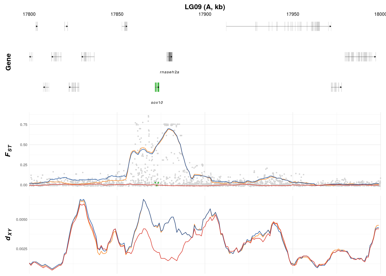
Here we apply the create_K_plot() function one for every subplot (a,b,c & d). Within the function we specify the current LG, the annotation file, the extend of the region in question, candidate genes, genes of secondary interest, SNP positions of interest, and the outlier region ID as defined in Figure 2.
p1 <- create_K_plot(searchLG = "LG09",gfffile = '../../1-output/09_gff_from_IKMB/HP.annotation.named.gff',xr = c(17800000,18000000),
                    searchgene = c("SOX10_1"),secondary_genes = c("RNASEH2A"),searchsnp = c(17871737,17872597,17873443),
                    muskID = 'A')
p2 <- create_K_plot(searchLG = "LG12",gfffile = '../../1-output/09_gff_from_IKMB/HP.annotation.named.gff',xr = c(20080000,20500000),
                    searchgene = c("Casz1_2"),secondary_genes = c(),searchsnp = c(20316944,20317120,20323661,20323670,20333895,20347263),
                    muskID = 'B')
p3 <- create_K_plot(searchLG = "LG12",gfffile = '../../1-output/09_gff_from_IKMB/HP.annotation.named.gff',xr = c(22100000,22350000),
                    searchgene = c("hoxc13a"),secondary_genes = c('hoxc10a',"hoxc11a","hoxc12a","calcoco1_1"),
                    searchsnp = c(),
                    muskID = 'C')
p4 <- create_K_plot(searchLG = "LG17",gfffile = '../../1-output/09_gff_from_IKMB/HP.annotation.named.gff',xr = c(22500000,22670000),
                    searchgene = c('LWS',"SWS2abeta","SWS2aalpha","SWS2b"),searchsnp = c(22553970,22561903,22566254),
                    secondary_genes = c("Hcfc1","HCFC1_2","HCFC1_1","GNL3L","TFE3_0","MDFIC2_1","CXXC1_3","CXXC1_1",'Mbd1','CCDC120'),
                    muskID = 'D')
An individual result will look like this (p1):
We read in the external legend:
legGrob <- gTree(children=gList(pictureGrob(readPicture("../../0_data/0_img/legend-pw-cairo.svg"))))And combine the individual subplots with the legend:
F3 <- plot_grid(NULL,NULL,NULL,NULL,
          p1,NULL,p2,NULL,
          NULL,NULL,NULL,NULL,
          p3,NULL,p4,NULL,
          NULL,NULL,NULL,NULL,
          ncol=4,rel_heights = c(.03,1,.03,1,.1),rel_widths = c(1,.025,1,.02),
          labels = c('a','','b','',
                     '','','','',
                     'c','','d','',
                     '','','','',
                     '','','',''),label_size = 10)+
  draw_grob(legGrob, 0.1, 0, .8, 0.04)
The final figure is then exported using ggsave().
ggsave(plot = F3, filename = '../output/F3.pdf',width = 183,height = 155,units = 'mm',device = cairo_pdf)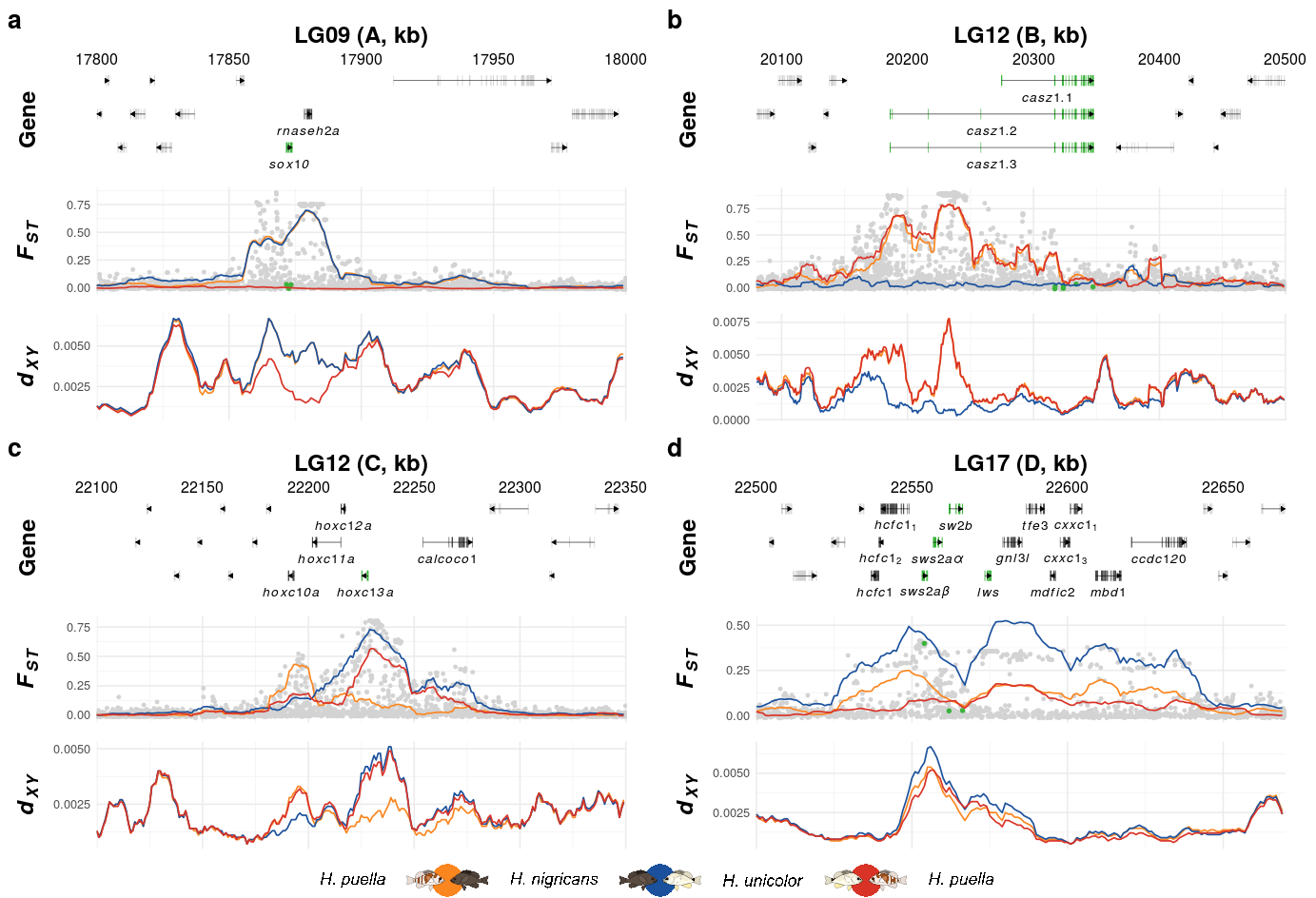
5.3 Details of F3.plot_fun.R
The actual work for figure 3 is done within the create_K_plot() function.
This function loads the data and does the plotting - the F3.R script is basically just a wrapper that selects the setting for each subplot and combines the results.
The function starts by importing the functions need to import the different data types (gene models, FST values, GxP p values, dXY)
create_K_plot <- function(searchLG,gfffile,xr,searchgene,secondary_genes,searchsnp,muskID){
  source('../../0_data/0_scripts/F3.functions.R');
  source('../../0_data/0_scripts/F3.getFSTs.R')
  source('../../0_data/0_scripts/F3.getDXY.R')
It then sets some global options for the plotting and throws an error if the genomic range is negative.
  highclr <- '#3bb33b'
  theme_set(theme_minimal(base_size = 6))
  if(xr[1]>xr[2]){print('error: ill conditioned x-range')}
  wdth <- .3
Then the different data types are imported using the previously loaded import functions.
  # get gene models
  df_list <- get_anno_df_single_line(searchLG=searchLG,gfffile=gfffile,xrange=xr,
                                     genes_of_interest = searchgene,genes_of_sec_interest=secondary_genes,anno_rown=3)

  # get fst values
  fst_list <- getFSTS(searchLG,xr,searchsnp,highclr)
  global_fst<-fst_list$global_fst;
  data_fst<-fst_list$data_fst

  # get dxy values
  dxy_list <- getDXY(searchLG,xr)
  data_dxy<-dxy_list$data_dxy
Then the color themes, axis labels further global plotting settings are set.
  clr <- c('#fb8620','#1b519c','#d93327')
  annoclr <- c('lightgray',highclr,rgb(.3,.3,.3))[1:3]
  df_list[[1]] <- df_list[[1]] %>% mutate(label=paste("italic(",tolower(Parentgenename),")",sep='') )
  LW <- .3;lS <- 9;tS <- 6
  plotSET <-  theme(rect = element_blank(),
                    text=element_text(size=tS,color='black'),
                    panel.grid.major = element_line(colour = rgb(.92,.92,.92)),
                    panel.grid.minor = element_line(colour = rgb(.95,.95,.95)),
                    plot.background = element_blank(),
                    plot.margin = unit(c(3,7,3,3),'pt'),
                    panel.background = element_blank(),#element_rect(colour = 'gray',fill=NULL),
                    legend.position = 'none',#c(.8,.3),
                    legend.direction = 'horizontal',
                    axis.title.y = element_blank(),
                    axis.title.x = element_blank(),#element_text(size=13,face='bold',color='black'),
                    strip.text.y = element_text(size=lS,color='black'),
                    axis.text.x = element_blank(),#element_text(size=11,color='black'),
                    strip.placement = "outside",
                    panel.border = element_blank()
  )
The individual data tracks are then plotted individually. Later the single tracks are aligned.
The first data track contains the gene models from the annotation file as well as the x axis labels (the position on the current LG).
  p11 <- ggplot()+
    # setting the genomic range
    coord_cartesian(xlim=xr/1000)+
    # including the exons as blocks
    geom_rect(data=df_list[[2]],aes(xmin=ps/1000,xmax=pe/1000,ymin=yl-(wdth/2),ymax=yl+(wdth/2),
                                    fill=as.factor(clr),col=as.factor(clr),group=Parent),lwd=.1)+
    # including the extend and direction of each mRNA
    geom_segment(data=(df_list[[1]]%>%filter(strand%in%c('+','-'))),
                 aes(x=ps/1000,xend=pe/1000,y=yl,yend=yl,group=Parent),lwd=.1,
                 arrow=arrow(length=unit(2,"pt"),type='closed'),color='black')+
    # including the extend of mRNA (if direction is unknown)
    geom_segment(data=(df_list[[1]]%>%filter(!strand%in%c('+','-'))),
                 aes(x=ps/1000,xend=pe/1000,y=yl,yend=yl,group=Parent),lwd=.2,color='black')+
    # include gene name as label
    geom_text(data=(df_list[[1]]%>%filter(Parentgenename%in%c(searchgene,secondary_genes))),
              aes(x=labelx/1000,label=label,y=yl-.5),size=1.8,parse=T)+
    # this inhereted from ealier versions but kept to allow propper alignment with the other data tracks
    facet_grid(window~.,scales='free_y',
               switch = 'y',labeller = label_parsed,as.table = T)+
    # color settings
    scale_color_manual(values=annoclr,breaks=c("x","y","z"),guide=F)+
    scale_fill_manual(values=annoclr,guide=F)+
    # axes labels and settings
    scale_x_continuous(name=paste0(searchLG,' (',muskID,', kb)'),expand=c(0,0),position = 'top')+
    scale_y_continuous(breaks = seq(0,.75,length.out = 4))+
    # plot format adjustments
    theme(rect = element_blank(),
          text=element_text(size=tS,color='black'),
          panel.grid.major = element_blank(),
          panel.grid.minor = element_blank(),
          plot.background = element_blank(),
          panel.background = element_blank(),
          legend.position = c(.8,.3),
          legend.direction = 'horizontal',
          axis.title.y = element_blank(),
          axis.title.x = element_text(size=lS,face='bold',color='black'),
          strip.text.y = element_text(size=lS,color='black'),
          axis.text.x = element_text(size=tS,color='black'),
          strip.placement = "outside",
          panel.border = element_blank());
To achieve proper formatting, the gene labels are adjusted independently depending on the outlier region ID. This is done after plotting to be able to represent special formats within the plot labels (eg. Greek letters AND italics)
 if(muskID=='a'){
   p11$layers[[4]]$data$label <- c("italic(sox10)","italic(rnaseh2a)")
 } else if(muskID=='b'){
     p11$layers[[4]]$data$label <- c("italic(casz1^3)","italic(casz1^2)","italic(casz1^1)")
   } else if(muskID=='c'){
     p11$layers[[4]]$data$label <- c('italic(hoxc10a)',"italic(hoxc11a)","italic(hoxc12a)","italic(hoxc13a)","italic(calcoco1)")
   }else if(muskID=='e'){
     p11$layers[[4]]$data$label <- c("italic(polr1d)","italic(ednrb)")
   } else if(muskID=='f'){
     p11$layers[[4]]$data$label <- c("italic(foxd3)","italic(alg6)","italic(efcab7)")
   }  else if(muskID=='d'){
       p11$layers[[4]]$data$label <- c("italic(hcfc1)","italic(hcfc1[2])","italic(hcfc1[1])",'italic(paste(sws2a,"\u03B2"))',
                                       'italic(paste(sws2a,"\u03B1"))',"italic(sw2b)","italic(lws)",
                                       "italic(gnl3l)","italic(tfe3)","italic(mdfic2)","italic(cxxc1[3])",
                                       "italic(cxxc1[1])",'italic(mbd1)','italic(ccdc120)')
   }else if(muskID=='g'){
     p11$layers[[4]]$data$label <- c("italic(lgals3bpb)","italic(mpnd)","italic(sh3gl1)","italic(rorb)")
   }else if(muskID=='h'){
     p11$layers[[4]]$data$label <- c("italic(alg2)","italic(sec61b)","italic(nr4a3)",
                                        "italic(stx17)","italic(erp44)","italic(invs)")
   }
The second data track contains the FST values.
  p12 <-  ggplot()+
    # setting the genomic range
    coord_cartesian(xlim = xr)+
    # including the global Fst values (SNP) basis
    geom_point(data = global_fst, aes(x = POS, y = WEIR_AND_COCKERHAM_FST), col = global_fst$clr, size = .2)+
    # highlight the SNPs of interest
    geom_point(data = global_fst, aes(x = POS, y = WEIR_AND_COCKERHAM_FST), col = global_fst$clr2, size = .3)+
    # add pairwise fsts as lines (10 kb / 1kb)
    geom_line(data = (data_fst %>% filter(POS > xr[1],POS<xr[2]))
              ,aes(x = POS, y = WEIGHTED_FST, col = run), lwd = LW)+
    # set color theme
    scale_color_manual(values = c(clr, annoclr), breaks = c("nig-pue", "nig-uni", "pue-uni"), guide = F)+
    scale_fill_manual(values = annoclr, guide = F)+
    # this inhereted from ealier versions but kept to allow propper alignment with the other data tracks
    facet_grid(window~., scales = 'free_y',
               switch = 'y', labeller = label_parsed, as.table = T)+
    # axes settings
    scale_x_continuous(name = searchLG, expand = c(0, 0), position = 'top')+
    scale_y_continuous(breaks = seq(0, .75, length.out = 4))+
    scale_linetype(name = 'location', label = c('Belize', 'Honduras','Panama'))+
    guides(linetype= guide_legend(override.aes = list(color = 'black')))+
    # include pre-set plot theme
    plotSET
The third data track contains the dXY values.
  p13 <-  ggplot()+
    # setting the genomic range
    coord_cartesian(xlim=xr)+
    geom_line(data=(data_dxy %>% filter(POS > xr[1],POS<xr[2]))
              ,aes(x=POS,y=dxy,col=run),lwd=LW)+
    # geom_line(data=(data_dxy_pw %>% filter(POS > xr[1],POS<xr[2]))
    #            ,aes(x=POS,y=dxy,col=run,linetype=group),lwd=1)+
    scale_color_manual(values=c(clr,annoclr),breaks=c("nig-pue","nig-uni","pue-uni","x","y","z"),guide=F)+
    # this inhereted from ealier versions but kept to allow propper alignment with the other data tracks
    facet_grid(window~.,scales='free_y',
               switch = 'y',labeller = label_parsed,as.table = T)+
    # axes settings
    scale_x_continuous(name=searchLG,expand=c(0,0),position = 'top')+
    scale_y_continuous(breaks = seq(0,.01,length.out = 5))+
    scale_linetype(name='location',label=c('Belize','Honduras','Panama'))+
    guides(linetype= guide_legend(override.aes = list(color = 'black')))+
    # include pre-set plot theme
    plotSET
Finally the individual tracks are stacked and aligned using plot_grid() (cowplot package). The complete sub figure is then returned by the function.
  p2 <- plot_grid(p11,p12,p13,
                  ncol = 1,align = 'v',axis = 'r',rel_heights = c(1.3,rep(1,2)))
  return(p2)}