4 Figure 2
4.1 Summary
This is the accessory documentation of Figure 2.
The Figure can be recreated by running the R script F2.R:
cd $WORK/3_figures/F_scripts

Rscript --vanilla F2.R
rm Rplots.pdf
4.2 Details of F2.R
In the following, the individual steps of the R script are documented. Is an executable R script that depends on a variety of image manipulation and data managing packages.
library(grid)
library(gridSVG)
library(grImport2)
library(grConvert)
library(tidyverse)
library(cowplot)
library(hrbrthemes)
4.2.1 Reading in Data
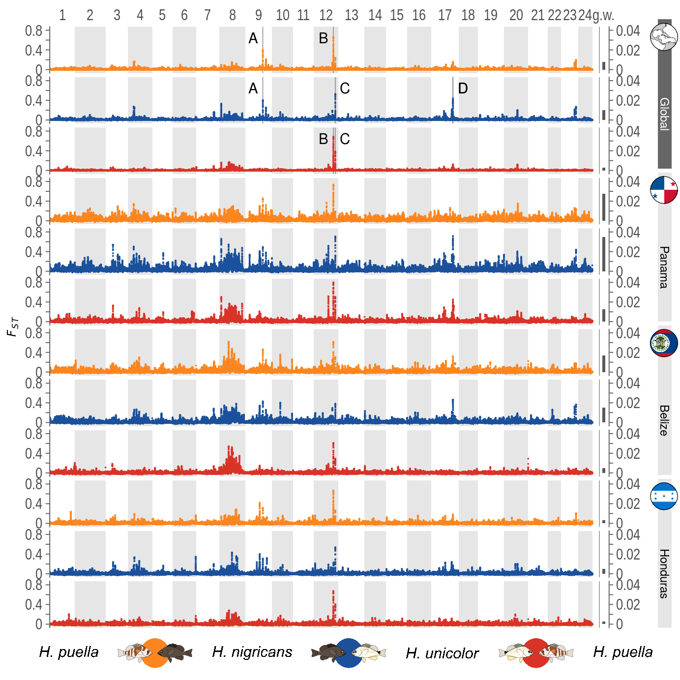
Figure 2 depends on the results of the FST computation by VCFtools in broad resolution (50 kb windows, 5 kb increments). The results of the individual species pairs are loaded individually, the genomic positions added to the loci and details about the species comparisons added.
Further more, the extent of the individual LGs in loaded.
karyo <- read.csv('../../0_data/0_resources/F2.karyo.txt',sep='\t') %>%
  mutate(GSTART=lag(cumsum(END),n = 1,default = 0),
         GEND=GSTART+END,GROUP=rep(letters[1:2],12)) %>%
  select(CHROM,GSTART,GEND,GROUP)

# Global -------------
pn <- read.csv('../../2_output/08_popGen/05_fst/pue-nig.50kb.5kb.windowed.weir.fst',sep='\t') %>%
   merge(.,(karyo %>% select(-GEND,-GROUP)),by='CHROM',allx=T) %>%
  mutate(POS=(BIN_START+BIN_END)/2,GPOS=POS+GSTART,COL='PN',RUN='PN');

pu <- read.csv('../../2_output/08_popGen/05_fst/pue-uni.50kb.5kb.windowed.weir.fst',sep='\t') %>%
  merge(.,(karyo %>% select(-GEND,-GROUP)),by='CHROM',allx=T) %>%
  mutate(POS=(BIN_START+BIN_END)/2,GPOS=POS+GSTART,COL='PU',RUN='PU');

nu <- read.csv('../../2_output/08_popGen/05_fst/nig-uni.50kb.5kb.windowed.weir.fst',sep='\t') %>%
  merge(.,(karyo %>% select(-GEND,-GROUP)),by='CHROM',allx=T) %>%
  mutate(POS=(BIN_START+BIN_END)/2,GPOS=POS+GSTART,COL='NU',RUN='NU');
# Panama -------------
ppnp <- read.csv('../../2_output/08_popGen/05_fst/pueboc-nigboc.50kb.5kb.windowed.weir.fst',sep='\t') %>%
  merge(.,(karyo %>% select(-GEND,-GROUP)),by='CHROM',allx=T) %>%
  mutate(POS=(BIN_START+BIN_END)/2,GPOS=POS+GSTART,COL='PN',RUN='PPNP');

ppup <- read.csv('../../2_output/08_popGen/05_fst/pueboc-uniboc.50kb.5kb.windowed.weir.fst',sep='\t') %>%
  merge(.,(karyo %>% select(-GEND,-GROUP)),by='CHROM',allx=T) %>%
  mutate(POS=(BIN_START+BIN_END)/2,GPOS=POS+GSTART,COL='PU',RUN='PPUP');

npup <- read.csv('../../2_output/08_popGen/05_fst/nigboc-uniboc.50kb.5kb.windowed.weir.fst',sep='\t') %>%
  merge(.,(karyo %>% select(-GEND,-GROUP)),by='CHROM',allx=T) %>%
  mutate(POS=(BIN_START+BIN_END)/2,GPOS=POS+GSTART,COL='NU',RUN='NPUP');
# Belize -------------
pbnb <- read.csv('../../2_output/08_popGen/05_fst/puebel-nigbel.50kb.5kb.windowed.weir.fst',sep='\t') %>%
  merge(.,(karyo %>% select(-GEND,-GROUP)),by='CHROM',allx=T) %>%
  mutate(POS=(BIN_START+BIN_END)/2,GPOS=POS+GSTART,COL='PN',RUN='PBNB');

pbub <- read.csv('../../2_output/08_popGen/05_fst/puebel-unibel.50kb.5kb.windowed.weir.fst',sep='\t') %>%
  merge(.,(karyo %>% select(-GEND,-GROUP)),by='CHROM',allx=T) %>%
  mutate(POS=(BIN_START+BIN_END)/2,GPOS=POS+GSTART,COL='PU',RUN='PBUB');

nbub <- read.csv('../../2_output/08_popGen/05_fst/nigbel-unibel.50kb.5kb.windowed.weir.fst',sep='\t') %>%
  merge(.,(karyo %>% select(-GEND,-GROUP)),by='CHROM',allx=T) %>%
  mutate(POS=(BIN_START+BIN_END)/2,GPOS=POS+GSTART,COL='NU',RUN='NBUB');
# Honduras -------------
phnh <- read.csv('../../2_output/08_popGen/05_fst/puehon-nighon.50kb.5kb.windowed.weir.fst',sep='\t') %>%
  merge(.,(karyo %>% select(-GEND,-GROUP)),by='CHROM',allx=T) %>%
  mutate(POS=(BIN_START+BIN_END)/2,GPOS=POS+GSTART,COL='PN',RUN='PHNH');

phuh <- read.csv('../../2_output/08_popGen/05_fst/puehon-unihon.50kb.5kb.windowed.weir.fst',sep='\t') %>%
  merge(.,(karyo %>% select(-GEND,-GROUP)),by='CHROM',allx=T) %>%
  mutate(POS=(BIN_START+BIN_END)/2,GPOS=POS+GSTART,COL='PU',RUN='PHUH');

nhuh <- read.csv('../../2_output/08_popGen/05_fst/nighon-unihon.50kb.5kb.windowed.weir.fst',sep='\t') %>%
  merge(.,(karyo %>% select(-GEND,-GROUP)),by='CHROM',allx=T) %>%
  mutate(POS=(BIN_START+BIN_END)/2,GPOS=POS+GSTART,COL='NU',RUN='NHUH');
The individual species comparisons are combined into a single data set. Then the order of the species comparisons and of the comparison types are set.
data <- rbind(pn,pu,nu,ppnp,ppup,npup,pbnb,pbub,nbub,phnh,phuh,nhuh)
data$RUN <- factor(as.character(data$RUN),
                   levels=c('PN','NU','PU','PPNP','NPUP','PPUP','PBNB','NBUB','PBUB','PHNH','NHUH','PHUH'))
data$COL <- factor(as.character(data$COL),levels=c('PN','PU','NU'))
Then, the genome wide weighted mean of FST is loaded.
gwFST <- read.csv('../../2_output/08_popGen/05_fst/genome_wide_weighted_mean_fst.txt',sep='\t')
gwFST$RUN <- factor(gwFST$run,levels=levels(data$RUN))
4.2.2 Computing 99.98 FST percentiles
The upper 99.98 FST percentile is computed per run. Then windows above this threshold are identified for each global run.
threshs <- data %>% group_by(RUN) %>% summarise(thresh=quantile(WEIGHTED_FST,.9998))

data2 <- data %>%
  filter(RUN %in% levels(data$RUN)[1:3]) %>%
  merge(.,threshs,by='RUN',all.x=T) %>%
  mutate(OUTL = (WEIGHTED_FST>thresh)) %>%
  filter(OUTL) %>%
  group_by(RUN) %>%
  mutate(CHECK=cumsum(1-(BIN_START-lag(BIN_START,default = 0)==5000)),ID=paste(RUN,'-',CHECK,sep='')) %>%
  ungroup() %>%
  group_by(ID) %>%
  summarise(CHROM=CHROM[1],
            xmin = min(BIN_START+GSTART),
            xmax=max(BIN_END+GSTART),
            xmean=mean(GPOS),
            LGmin=min(BIN_START),
            LGmax=min(BIN_END),
            LGmean=min(POS),
            RUN=RUN[1],COL=COL[1]) %>%
  ungroup() %>% mutate(muskS = letters[as.numeric(as.factor(xmin))],
                       musk=LETTERS[c(1,3,4,4,1,2,2,3)])

musks <- data2 %>% group_by(musk) %>% summarise(MUSKmin=min(xmin),
                                                MUSKmax=max(xmax),
                                                MUSKminLG=min(LGmin),
                                                MUSKmaxLG=max(LGmax)) %>%
  merge(data2,.,by='musk') %>% mutate(muskX = ifelse(musk %in% c("A","B"),
                                                     MUSKmin-1e+07,MUSKmax+1e+07))
4.2.3 Plotting
For plotting, colors,labels and the scaling of the secondary axis are pre-defined.
clr <- c('#fb8620','#d93327','#1b519c')
annoclr <- rgb(.4,.4,.4)
lgclr <- rgb(.9,.9,.9)

yl <- expression(italic('F'[ST]))
secScale <- 20
The base plot is done with ggplot().
p1 <- ggplot()+
  # background shading for LGs
  geom_rect(inherit.aes = F,data=karyo,aes(xmin=GSTART,xmax=GEND,
                                           ymin=-Inf,ymax=Inf,fill=GROUP))+
  # vertical lines for outlier windows
  geom_vline(data=data2,aes(xintercept=xmean),col=annoclr,lwd=.2)+
  # Fst values
  geom_point(data=data,aes(x=GPOS,y=WEIGHTED_FST,col=COL),size=.01)+
  # labels for the outlier windows
  geom_text(data=musks,aes(x=muskX,y=.65,label=musk))+
  # vertical line separating sliding Fst from genome wide Fst
  geom_vline(data = data.frame(x=567000000),aes(xintercept=x),col=annoclr,lwd=.2)+
  # genome wide Fst
  geom_rect(data=gwFST,aes(xmin=570*10^6,xmax=573*10^6,ymin=0,ymax=gwFST*secScale))+
  # layout of y axis and secondary y axis
  scale_y_continuous(name = yl,limits=c(-.03,.83),
                     breaks=0:4*0.2,labels = c(0,'',0.4,'',0.8),
                     sec.axis = sec_axis(~./secScale,labels = c(0,'',.02,'',.04)))+
  # layout of x axis
  scale_x_continuous(expand = c(0,0),limits = c(0,577*10^6),
                     breaks = c((karyo$GSTART+karyo$GEND)/2,571*10^6),
                     labels = c(1:24,"g.w."),position = "top")+
  # set color map
  scale_color_manual(name='comparison',values=clr)+
  # set fill of LG backgrounds
  scale_fill_manual(values = c(NA,lgclr),guide=F)+
  # pre-defined plot theme
  theme_ipsum(grid = F,
              axis_title_just = 'c',
              axis_title_family = 'bold',
              strip_text_size = 9)+
  # tweaks of the plot theme
  theme(plot.margin = unit(c(2,25,40,0),'pt'),
        panel.spacing.y = unit(3,'pt'),
        legend.position = 'none',
        axis.title.x = element_blank(),
        axis.ticks.y = element_line(color = annoclr),
        axis.line.y =  element_line(color = annoclr),
        axis.text.y = element_text(margin = unit(c(0,3,0,0),'pt')),
        axis.title.y = element_text(vjust = -1),
        strip.background = element_blank(),
        strip.text = element_blank())+
  # separate the plots of the individual species pairs
  facet_grid(RUN~.)
External images are loaded for annotation.
legGrob <- gTree(children=gList(pictureGrob(readPicture("../../0_data/0_img/legend-pw-cairo.svg"))))
carGrob <- gTree(children=gList(pictureGrob(readPicture("../../0_data/0_img/caribbean-cairo.svg"))))
panGrob <- gTree(children=gList(pictureGrob(readPicture("../../0_data/0_img/panama-cairo.svg"))))
belGrob <- gTree(children=gList(pictureGrob(readPicture("../../0_data/0_img/belize-cairo.svg"))))
honGrob <- gTree(children=gList(pictureGrob(readPicture("../../0_data/0_img/honduras-cairo.svg"))))
# variables for annotation placement
ys <- .0765
ysc <- .0057
yd <- .2195
boxes = data.frame(x=rep(.9675,4),y=c(ys,ys+yd+ysc,ys+(yd+ysc)*2,ys+(yd+ysc)*3))
4.2.4 Composing the final figure
And finally the base plot is combined with the external annotations.
F2 <- ggdraw(p1)+
  geom_rect(data = boxes, aes(xmin = x, xmax = x + .02, ymin = y, ymax = y + yd),
            colour = NA, fill = c(rep(lgclr,3),annoclr))+
  draw_label('Global', x = .9775, y = boxes$y[4]+.08,
             size = 9, angle=-90,col='white')+
  draw_label('Belize', x = .9775, y = boxes$y[2]+.08,
             size = 9, angle=-90)+
  draw_label('Honduras', x = .9775, y = boxes$y[1]+.08,
             size = 9, angle=-90)+
  draw_label('Panama', x = .9775, y = boxes$y[3]+.08,
              size = 9, angle=-90)+
  draw_grob(legGrob, 0.01, 0, 1, 0.08)+
  draw_grob(carGrob, 0.954, boxes$y[4]+.78*yd, .045, .045)+
  draw_grob(belGrob, 0.954, boxes$y[2]+.78*yd, .045, .045)+
  draw_grob(honGrob, 0.954, boxes$y[1]+.78*yd, .045, .045)+
  draw_grob(panGrob, 0.954, boxes$y[3]+.78*yd, .045, .045)
The FST outlier windows are then exported to be used as reference in other figures.
write.table(x = data2, file = '../../0_data/0_resources/fst_outlier_windows.txt',sep='\t',quote = F,row.names = F)
write.table(x = musks, file = '../../0_data/0_resources/fst_outlier_ID.txt',sep='\t',quote = F,row.names = F)
The figure is then exported using ggsave().
ggsave(plot = F2,filename = '../output/F2.png',width = 183,height = 183,dpi = 200,units = 'mm')
#ggsave('fst_mac02_weight_99.98.eps',width = 183,height = 183,dpi = 200,units = 'mm')