13 Supplementary Figure 08

13.1 Summary

This is the accessory documentation of Supplementary Figure 08.

The Figure can be recreated by running the R script S08.R:

cd $WORK/3_figures/F_scripts

Rscript --vanilla S08.R
rm Rplots.pdf

13.2 Details of S08.R

The S08.R script is basically a variant of the F3.R script. Is an executable R script that depends on a variety of image manipulation and data managing and genomic data packages.

It Furthermore depends on the R scripts S08.plot_fun.R which itselve depends on S08.functions.R and F3.getFSTs.R (all located under $WORK/0_data/0_scripts).

library(grid)
library(gridSVG)
library(grImport2)
library(grConvert)
library(tidyverse)
library(rtracklayer)
library(hrbrthemes)
library(cowplot)
require(rtracklayer)

source('../../0_data/0_scripts/S08.plot_fun.R')

The extend of the outlierredion is read in and the margin to plot on either side of the outlier regions is defined.

dat <- read.csv('../../0_data/0_resources/outlier_regions.bed',sep='\t',header = FALSE,stringsAsFactors = FALSE)
mar <- 10^5

Then the labels of the individual regions are set:

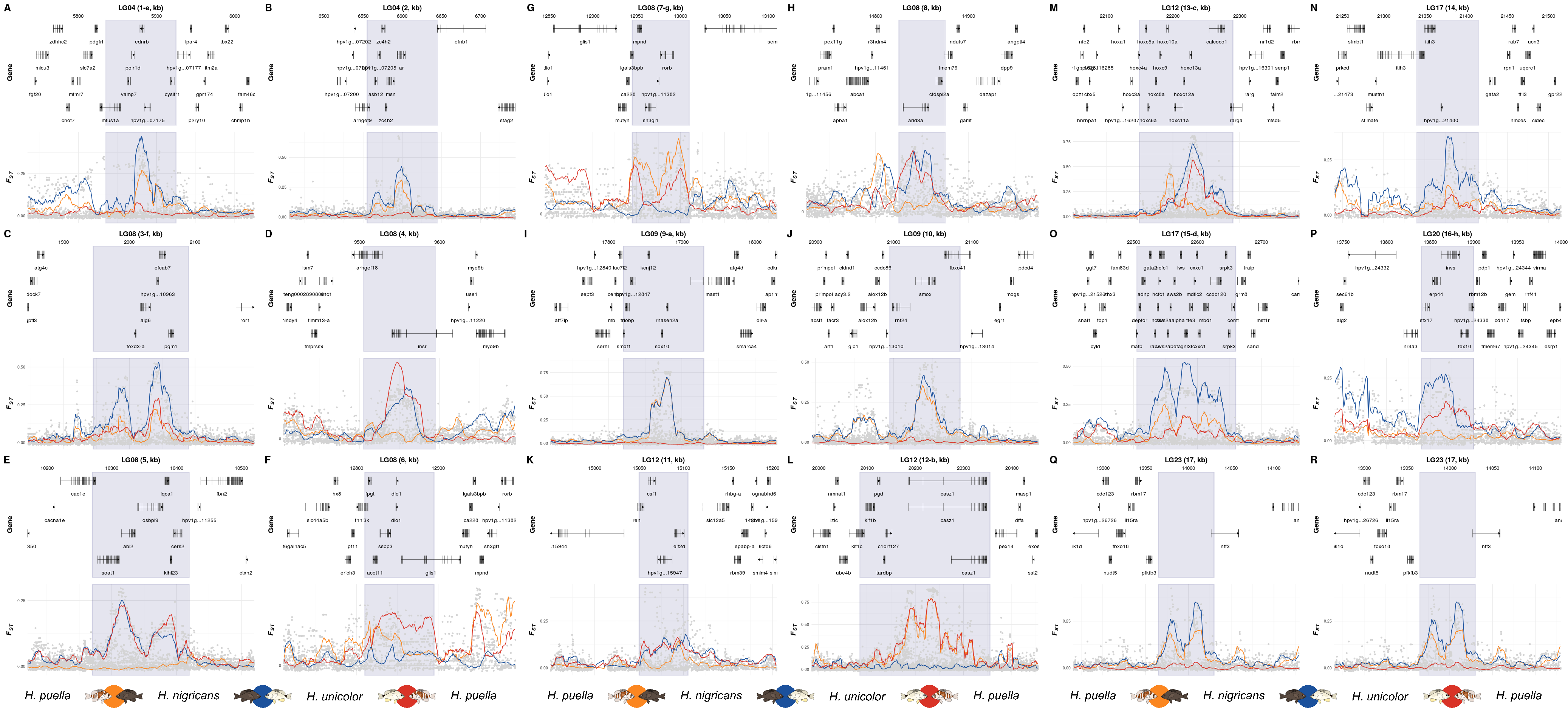
mI <- c('-e','','-f',rep('',3),'-g','','-a',rep('',2),'-b','-c','','-d','-h',rep('',2))

Within one loop, each outlier region is plotted using the create_K_plot() function and the plots are stored within a list.

plts <- list()
for(k in 1:18){
  print(k)
  x1 <- dat$V2[k]
  x2 <- dat$V3[k]
  plts[[k]] <- create_K_plot(searchLG = dat$V1[k],
                             gfffile = '../../1-output/09_gff_from_IKMB/HP.annotation.named.gff',
                             xr = c(x1-mar,x2+mar),
                             xr2=c(x1,x2),
                             muskID = paste0(k,mI[k]))
}

Then the legend of the plots is read in.

legGrob <- gTree(children=gList(pictureGrob(readPicture("../../0_data/0_img/legend-pw-cairo.svg"))))

The three subfigures (Supplementary Figure 08 I, II & III) are composed of six plots each plus the legend.

p1 <- plot_grid(plts[[1]],plts[[2]],
                plts[[3]], plts[[4]],
                plts[[5]],plts[[6]],
                labels=LETTERS[1:6],label_size = 10,
                ncol=2)
S08a <- ggdraw()+
  draw_plot(p1,0,.05,1,.95)+
  draw_plot(legGrob,0,0,1,.05)

p2 <- plot_grid(plts[[7]],plts[[8]],
                plts[[9]], plts[[10]],
                plts[[11]],plts[[12]],
                labels=LETTERS[7:12],label_size = 10,
                ncol=2)

S08b <- ggdraw()+
  draw_plot(p2,0,.05,1,.95)+
  draw_plot(legGrob,0,0,1,.05)

p3 <- plot_grid(plts[[13]],plts[[14]],
                plts[[15]], plts[[16]],
                plts[[17]],plts[[17]],
                labels=LETTERS[13:18],label_size = 10,
                ncol=2)
S08c <- ggdraw()+
  draw_plot(p3,0,.05,1,.95)+
  draw_plot(legGrob,0,0,1,.05)

Finally, the subfigures are exported using ggsave().

ggsave(plot = S08a,filename = '../output/S08a.pdf',width = 183,height = 250,units = 'mm',device = cairo_pdf)
ggsave(plot = S08b,filename = '../output/S08b.pdf',width = 183,height = 250,units = 'mm',device = cairo_pdf)
ggsave(plot = S08c,filename = '../output/S08c.pdf',width = 183,height = 250,units = 'mm',device = cairo_pdf)

---