9 Supplementary Figure 03

9.1 Summary

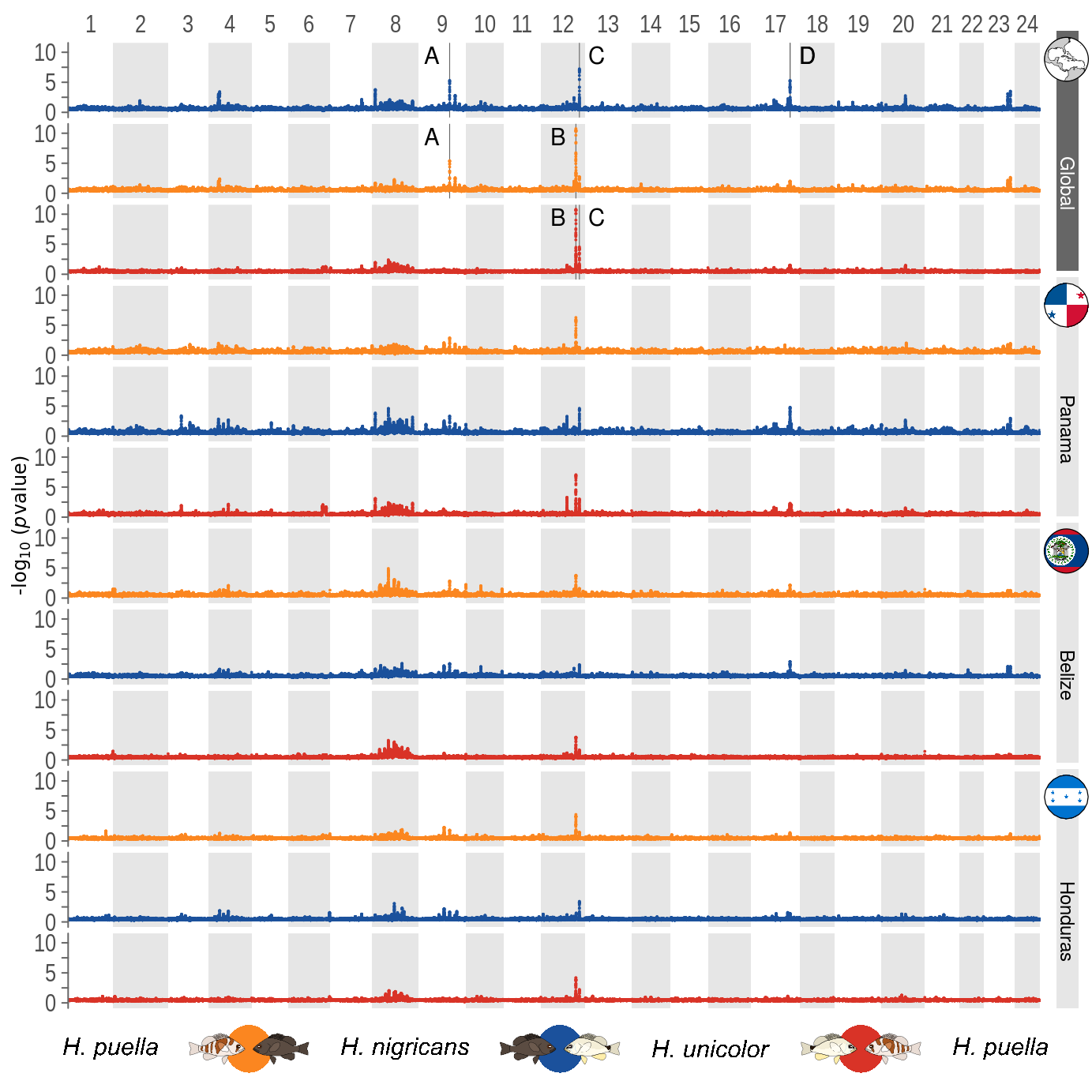
This is the accessory documentation of Supplementary Figure 03.

The Figure can be recreated by running the R script S03.R:

cd $WORK/3_figures/F_scripts

Rscript --vanilla S03.R
rm Rplots.pdf

9.2 Details of S03.R

In principal the S03.R script is a reduced versions of the F2.R script. Is an executable R script that depends on a variety of image manipulation and data managing packages.

In the following the differences to F3.R are highlighted. Obvious changes (different data input files, axis labels, y range) are omitted.

Apart from these trivial changes, the genome wide summary of the statistic is omitted.

Therefore, the following lines of the original Script (F2.R) were removed from S03.R:

gwFST <- read.csv('../../2_output/08_popGen/05_fst/genome_wide_weighted_mean_fst.txt',sep='\t')
gwFST$RUN <- factor(gwFST$run,levels=levels(data$RUN))
#....#
p1 <- ggplot()+
#....#
 geom_vline(data = data.frame(x=567000000),aes(xintercept=x),col=annoclr,lwd=.2)+
 geom_rect(data=gwFST,aes(xmin=570*10^6,xmax=573*10^6,ymin=0,ymax=gwFST*secScale))+
#....#

Furthermore, the generation of the outlier annotation changed. While in the F_ST script, the outlier where determined from the loaded data and later exported, within the G x P script the the highlights don’t refer to G x P outliers, but the old F_ST outlier are imported and plotted for reference.

data2 <- read.csv('../../0_data/0_resources/fst_outlier_windows.txt', sep='\t')
musks <- read.csv('../../0_data/0_resources/fst_outlier_ID.txt', sep='\t')

This replaced the original section that computes the outlier windows within F2.R:

threshs <- data %>% group_by(RUN) %>% summarise(thresh=quantile(WEIGHTED_FST,.9998))

data2 <- data %>% filter(RUN %in% levels(data$RUN)[1:3]) %>% merge(.,threshs,by='RUN',all.x=T) %>%
  mutate(OUTL = (WEIGHTED_FST>thresh)) %>% filter(OUTL) %>% group_by(RUN) %>%
  mutate(CHECK=cumsum(1-(BIN_START-lag(BIN_START,default = 0)==5000)),ID=paste(RUN,'-',CHECK,sep='')) %>%
  ungroup() %>% group_by(ID) %>%
  summarise(CHROM=CHROM[1],
            xmin = min(BIN_START+GSTART),
            xmax=max(BIN_END+GSTART),
            xmean=mean(GPOS),
            LGmin=min(BIN_START),
            LGmax=min(BIN_END),
            LGmean=min(POS),
            RUN=RUN[1],COL=COL[1]) %>%
  ungroup() %>% mutate(muskS = letters[as.numeric(as.factor(xmin))],
                       musk=LETTERS[c(1,3,4,4,1,2,2,3)])

musks <- data2 %>% group_by(musk) %>% summarise(MUSKmin=min(xmin),
                                                MUSKmax=max(xmax),
                                                MUSKminLG=min(LGmin),
                                                MUSKmaxLG=max(LGmax)) %>%
  merge(data2,.,by='musk') %>% mutate(muskX = ifelse(musk %in% c("A","B"),
                                                     MUSKmin-1e+07,MUSKmax+1e+07))

The final plot, as produced by the S03.R script:

---