8 Supplementary Figure 02
8.1 Summary
This is the accessory documentation of Supplementary Figure 02.
The Figure can be recreated by running the R script S02.R:
cd $WORK/3_figures/F_scripts

Rscript --vanilla S02.R
rm Rplots.pdf
8.2 Details of S02.R
In the following, the individual steps of the R script are documented. Is an executable R script that depends on a variety of image manipulation and data managing.
It Furthermore depends on the R scripts S02.functions.R (located under $WORK/0_data/0_scripts).
library(grid)
library(gridSVG)
library(grImport2)
library(tidyverse)
library(RColorBrewer)
library(cowplot)
library(ggrepel)
source('../../0_data/0_scripts/S02.functions.R')
In the first step, the individual NewHybrids runs including the specificatioin of population 1 and population 2 are initialized. Then the results of the individual runs are loaded and merged. To import the posterior probability estiates the function getPofZ() from the helper script (S02.functions.R) is used. The hybridization class is then transformed into a factor.
run_list <- c("nigbel-puebel","nigbel-unibel","puebel-unibel",
              "nigboc-pueboc","nigboc-uniboc","pueboc-uniboc",
              "nighon-puehon","nighon-unihon","puehon-unihon")

pops_list <- data.frame(pop1=c('pue','nig','pue','nig','uni','pue','pue','nig','pue'),
                        pop2=c('nig','uni','uni','pue','nig','uni','nig','uni','uni'),
                        stringsAsFactors = F)

pop_order <- c(-1,-1,1,1,-1,-1,1,1,-1)
data <- data.frame(IndivName=c(), spec=c(),pop=c(), BIN=c(),
                   post_prob=c(),RUN=c(),stringsAsFactors = F)

for (k in 1:9) {
  data <- rbind(data,getPofZ(runname = run_list[k],
                             pops = pops_list[k,order((1:2)*pop_order[k])]))
}

data$BIN <- factor(as.character(data$BIN),
                   levels = c("F1","F2","nigPure","nigBC",
                              "puePure","pueBC","uniPure","uniBC"))
Annotations that are use within the individual plots are loaded andstored within a list.
pnGrob <- gTree(children=gList(pictureGrob(readPicture("../../0_data/0_img/pue-nig-rot-cairo.svg"))))
nuGrob <- gTree(children=gList(pictureGrob(readPicture("../../0_data/0_img/nig-uni-rot-cairo.svg"))))
upGrob <- gTree(children=gList(pictureGrob(readPicture("../../0_data/0_img/uni-pue-rot-cairo.svg"))))

gl <- list(pnGrob, nuGrob, upGrob)
The function plot_fun() (from the helper script S02.functions.R) is used to plot the NewHybrids results for each location.
pbel <- plot_fun(data,'bel',1, gl)
phon <- plot_fun(data,'hon',2, gl)
pboc <- plot_fun(data,'boc',3, gl)
Then some preparation is done for the pca plots. The colors are predefined, the sample metadata and the pca results are loaded and the introgression candidates are specified.
clr<-c('#000000','#d45500','#000000')
fll<-c('#000000','#d45500','#ffffff')

dataAll <- read.csv('../../0_data/0_resources/F1.sample.txt',sep='\t') %>%
  mutate(loc=substrRight(as.character(id),3))
belPCA <- readRDS('../../2_output/08_popGen/04_pca/bel/belpca.Rds')
honPCA <- readRDS('../../2_output/08_popGen/04_pca/hon/honpca.Rds')
panPCA <- readRDS('../../2_output/08_popGen/04_pca/pan/panpca.Rds')

introgression_candidates <- c('18161','18178','18180','18267','18274','18276',
                              '20558','20633','27678')
The function plotPCA() (from the helper script S02.functions.R) is used to plot the pca for each location including the highlighted introgression candidates.
p1 <- plotPCA(pca=belPCA, dataAll=dataAll, locIN='bel',
        introgression_candidates=introgression_candidates, clr=clr, fll=fll)

p2 <- plotPCA(pca=honPCA, dataAll=dataAll, locIN='hon',
              introgression_candidates=introgression_candidates, clr=clr, fll=fll)

p3 <- plotPCA(pca=panPCA, dataAll=(dataAll %>% filter(spec!='gum')), locIN='boc',
             introgression_candidates=introgression_candidates, clr=clr, fll=fll)
The basic structure of the figure is created using the the plot_grid() function of the cowplot package.
cp1 <- plot_grid(pbel+theme(legend.position = 'none'),p1,
          phon+theme(legend.position = 'none'),p2,
          pboc+theme(legend.position = 'none'),p3,
          ncol = 2,rel_heights = c(1,1,1),
          rel_widths = c(0.65,0.35),
          labels=c('a','b',rep('',4)),
          label_size = 10);
Then, external annotations loaded and variables needed for the plot composition are created.
legGrob <- gTree(children=gList(pictureGrob(readPicture("../../0_data/0_img/legend_NH-cairo.svg"))))
belGrob <- gTree(children=gList(pictureGrob(readPicture("../../0_data/0_img/belize-cairo.svg"))))
honGrob <- gTree(children=gList(pictureGrob(readPicture("../../0_data/0_img/honduras-cairo.svg"))))
panGrob <- gTree(children=gList(pictureGrob(readPicture("../../0_data/0_img/panama-cairo.svg"))))

ys <- .005
ysc <- .008
yd <- .3025
labX <- .675
bclr <- rgb(.9,.9,.9)
boxes = data.frame(x=rep(labX-.015,3),
                   y=c(ys,ys+yd+ysc,ys+(yd+ysc)*2))
Finally, the complete Supplementary Figure 02 is put together.
S02 <- ggdraw()+
  geom_rect(data = boxes, aes(xmin = x, xmax = x + .03, ymin = y+.07, ymax = y + yd+c(.07,.07,.05)),
            colour = NA, fill = c(rep(bclr,3)))+
  draw_label('Belize', x = labX, y = boxes$y[3]+.20,
             size = 13, angle=-90)+
  draw_label('Honduras', x = labX, y = boxes$y[2]+.20,
             size = 13, angle=-90)+
  draw_label('Panama', x = labX, y = boxes$y[1]+.20,
             size = 13, angle=-90)+
  draw_label('Posterior probability',x=.01,y=.57,size = 15, angle=90)+
  draw_grob(legGrob,0,0,1,.07)+
  draw_plot(cp1,.0,.07,1,.93)+
  draw_grob(belGrob, labX-.0225, boxes$y[3]+.84*yd+.05, .045, .045)+
  draw_grob(honGrob, labX-.0225, boxes$y[2]+.84*yd+.07, .045, .045)+
  draw_grob(panGrob, labX-.0225, boxes$y[1]+.84*yd+.07, .045, .045)
The final figure is then exported using ggsave().
ggsave(plot = S02,filename = '../output/S02.pdf',width = 183,height = 235,units = 'mm',device = cairo_pdf)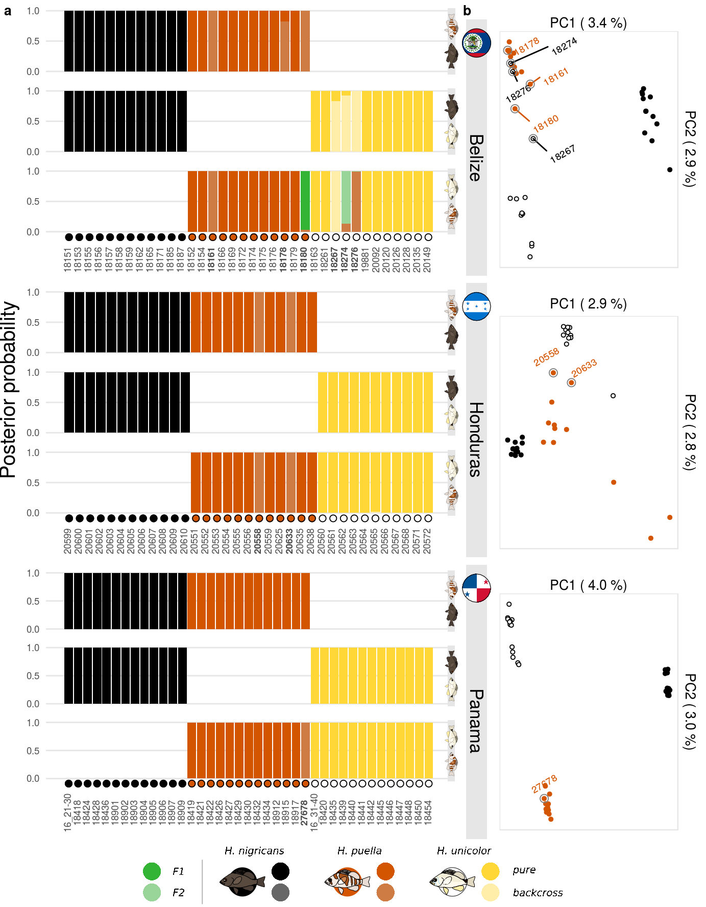
8.3 Details of S02.functions.R
This script contains the functions substrAllRight(),substrRight(),geom_custom(),getPofZ(),plot_fun(),plotPCA() and the objects theme_mapK and GeomCustom
The functions substrAllRight() and substrRight() are small sting manipulation functions that are used to format label within the plots.
substrAllRight <- function(x, n){substr(x, n+1, nchar(x))}
substrRight <- function(x, n){substr(x, nchar(x)-n+1, nchar(x))}
theme_mapK <- theme_minimal()+
theme(panel.grid = element_blank(),
text=element_text(size=10),
axis.text.y = element_text(size = 7),
axis.text.x = element_text(size = 7))This custom geom geom_custom (and GeomCustom) is copied fromm an by baptiste answer on github and is used to distribute the halet labels on the respective plot panels.
GeomCustom <- ggproto(
  "GeomCustom",
  Geom,
  setup_data = function(self, data, params) {
    data <- ggproto_parent(Geom, self)$setup_data(data, params)
    data
  },

  draw_group = function(data, panel_scales, coord) {
    vp <- grid::viewport(x=data$x, y=data$y)
    g <- grid::editGrob(data$grob[[1]], vp=vp)
    ggplot2:::ggname("geom_custom", g)
  },

  required_aes = c("grob","x","y")

)

geom_custom <-  function(mapping = NULL,
                         data = NULL,
                         stat = "identity",
                         position = "identity",
                         na.rm = FALSE,
                         show.legend = NA,
                         inherit.aes = FALSE,
                         ...) {
  layer(
    geom = GeomCustom,
    mapping = mapping,
    data = data,
    stat = stat,
    position = position,
    show.legend = show.legend,
    inherit.aes = inherit.aes,
    params = list(na.rm = na.rm, ...)
  )
}
The function getPofZ() is used to import the individual posterior probability estiates from the NewHybrids output. It also relabels the hybridisation classes based on the populations specified and adds the sample Ids.
getPofZ <- function(runname,pops){
  colN <- c(paste(c(pops[1],pops[1],pops[2],pops[2]),
                  c('Pure','BC','Pure','BC'),sep = ''))

  NHres <-read.csv(paste('../../2_output/08_popGen/11_newHyb/NH_PofZ/newHyb.',runname,'.txt_PofZ.txt',sep=''),sep='\t',
                   col.names = c('indNR','IndivName',
                                 colN[1],colN[3],
                                 'F1','F2',colN[2],colN[4]))

  NHres$IndivName <- read.csv(paste('../../2_output/08_popGen/11_newHyb/NH_PofZ/newHyb.',runname,'_individuals.txt',sep=''),
                              header = F,col.names = c('IndivName'))[,1] %>%
    as.character()

  IND_inventory <- read.csv('../../0_data/0_resources/sample_id.csv',sep='\t',header = F,
                            col.names = c('ID','IndivName','spec','pop','loc'),
                            stringsAsFactors = F)

  data <- NHres %>% merge(.,IND_inventory,by='IndivName',sort=F) %>%
    select(IndivName,spec,pop,one_of(colN[1],colN[3],'F1','F2',colN[2],colN[4])) %>%
    gather(key = 'BIN',value = "post_prob",4:9) %>%
    mutate(RUN=runname)

  return(data)
}
The function plot_fun() plots the NewHybrids results for sets of three pairwise comparisons within one location.
plot_fun <- function(data,loc,sel,gl){
  pdat <- data %>%
    filter(grepl(loc,RUN)) %>%
    arrange(spec,IndivName) %>%
    mutate(x2=paste0(spec,IndivName),x = as.numeric(as.factor(x2)))

  clr=c('#34b434','#99d499',
        '#000000',rgb(.4,.4,.4),
        "#d45500",'#cf7c44',
        '#ffd736','#ffeeaa')
  labsRAW <- substrAllRight(levels(as.factor(pdat$x2)),3)

  XL <- list(bel=expression('18151','18153','18155','18156','18157','18158','18159','18162','18165','18171',
                            '18185','18187','18152','18154',bold('18161'),'18166','18169','18172','18174',
                            '18175','18176',bold('18178'),'18179',bold('18180'),'18163','18261',bold('18267'),
                            bold('18274'),bold('18276'),'19881','20092','20120','20126','20128','20135','20149'),
             hon=expression('20599','20600','20601','20602','20603','20604','20605','20606','20607','20608',
                            '20609','20610','20551','20552','20553',bold('20554'),'20555','20556',
                            bold('20558'),bold('20559'),'20625',bold('20633'),'20635','20638','20560',
                            '20561','20562','20563','20564','20565','20566','20567','20568','20571','20572'),
             boc=expression("16_21-30","18418","18424","18428","18436","18901","18902","18903",
                             "18904","18905","18906","18907","18909","18419","18421","18422",
                             "18426","18427","18429","18430","18432","18434","18912","18915",
                             "18917",bold("27678"),"16_31-40","18420","18435","18439","18440","18441",
                             "18442","18445","18446","18447","18448","18450","18454"))

  groblist <- tibble(RUN=gsub('XX',loc,c('nigXX-pueXX','nigXX-uniXX','pueXX-uniXX')),
                     grob = gl )

  dotdat <- pdat %>%
    group_by(IndivName) %>%
    summarise(spec=spec[1],
              x=x[1],
              RUN=gsub('XX',loc,c('pueXX-uniXX')))
  Grobx=max(pdat$x)+1

  p <- ggplot(pdat,
              aes(x=x,fill=BIN))+
    facet_grid(RUN~.)+
    geom_hline(yintercept=c(0,.5,1),col=rgb(.9,.9,.9))+
    geom_custom(data=groblist, aes(grob=grob), inherit.aes = FALSE,
                x = 1, y=0.535)+
    geom_point(inherit.aes = F, data=dotdat,
               aes(x=x,y=-.09,col=spec),size=2)+
    geom_point(inherit.aes = F, data=dotdat,
               aes(x=x,y=-.09),col='black',size=2,shape=1)+
    geom_bar(aes(y=post_prob),stat = 'identity',position = "stack")+
    scale_fill_manual('class',values=clr)+
    scale_color_manual(values = c('#000000','#d45500','#ffffff'))+
    scale_y_continuous('',breaks = c(0,.5,1))+
    scale_x_continuous(breaks=1:(Grobx-1)-.5,labels=XL[[sel]])+
    theme_minimal()+
    theme(panel.grid = element_blank(),
          axis.text.y = element_text(size = 7),
          axis.text.x = element_text(angle = 90,size = 7),
          axis.title.x = element_blank(),
          legend.position = 'none',
          strip.background = element_blank(),
          strip.text = element_blank())

  return(p)
}
The function plotPCA() plots the pca results for one location and highlights the introgression candidates.
plotPCA <- function(pca,dataAll,locIN,introgression_candidates,clr,fll){
  data <- cbind(dataAll %>% filter(sample=='sample',loc==locIN) %>%
                  select(id,spec),
                  pca$scores);
  names(data)[3:12]<- paste('PC',1:10,sep='')
  exp_var <- (pca$singular.values[1:10])^2/length(pca$maf)
  xlab <- paste('PC1 (',sprintf("%.1f",exp_var[1]*100),'%)')# explained varinace)')
  ylab <- paste('PC2 (',sprintf("%.1f",exp_var[2]*100),'%)')# explained varinace)')
  p <- ggplot(data,aes(x=PC1,y=PC2,col=spec,fill=spec))+
    geom_point(size=1.1,shape=21)+
    geom_text_repel(inherit.aes = F,
                    data=(data %>% filter(gsub('[a-z,A-Z]','',id) %in% introgression_candidates)),
                    aes(x=PC1,y=PC2,col=spec,label=substr(id,1,5)),angle=30,size=2.5,nudge_y = .01)+
    geom_point(inherit.aes = F,data=(data %>% filter(gsub('[a-z,A-Z]','',id) %in% introgression_candidates)),
               aes(x=PC1,y=PC2),col=rgb(.5,.5,.5),size=2.5,shape=1)+
    scale_color_manual(values=clr,guide=F)+
    scale_fill_manual(values=fll,guide=F)+
    theme_mapK+
    theme(legend.position='bottom',
          panel.border = element_rect(color=rgb(.9,.9,.9),fill=rgb(1,1,1,0)),
          axis.title.y = element_text(vjust = -7),
          axis.title.x = element_text(vjust = 6),
          axis.text = element_blank(),
          plot.margin = unit(c(10,5,10,30),'pt'))+#coord_equal()+
    scale_x_continuous(name=xlab,breaks = c(-.2,.5),position = "top")+
    scale_y_continuous(name=ylab,breaks = c(-.4,.2),position = "right");
  return(p)
}