18 Supplementary Figure 13

18.1 Summary

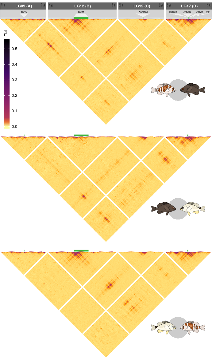
This is the accessory documentation of Supplementary Figure 13.

The Figure can be recreated by running the R script S13.R:

cd $WORK/3_figures/F_scripts

Rscript --vanilla S13.R
rm Rplots.pdf

18.2 Details of S13.R

In the following, the individual steps of the R script are documented. Is an executable R script that depends on a variety of image manipulation and data managing and genomic data packages.

It Furthermore depends on the R scripts F4.functions.R (located under $WORK/0_data/0_scripts).

This script is a modification of script F4.R. It uses the same functions and just differs in the data sets and settings

library(tidyverse)
library(scales)
library(cowplot)
library(grid)
library(gridSVG)
library(grImport2)
source('../../0_data/0_scripts/F4.functions.R')

The script F4.functions.Rcontains a function (trplot()) that plots a single LD triangle as seen in Supplementary Figure 13. The Details of this script are explained below. The output depends on the data set plotted (sub figure a contains additional annotations).

We create an empty list that is then filled with the subplots using the trplot() function.

plts <- list()

for(k in 1:3){
plts[[k]] <- trplot((8:10)[k])
}

The basic plots are transformed into grid obgects. These are afterwards rotated by 45 degrees.

tN <- theme(legend.position = 'none')

pG8 <- ggplotGrob(plts[[1]]+tN)
pG9 <- ggplotGrob(plts[[2]]+tN)
pG10 <- ggplotGrob(plts[[3]]+tN)
pGr8 <- editGrob(pG8, vp=viewport(x=0.5, y=0.97, angle=45,width = .76), name="pG8")
pGr9 <- editGrob(pG9, vp=viewport(x=0.5, y=0.62, angle=45,width = .7), name="pG9")
pGr10 <- editGrob(pG10, vp=viewport(x=0.5, y=0.3, angle=45,width = .7), name="pG10")

Then, external annotations loaded and the legend ins extracted from the first plot.

npGrob <- gTree(children=gList(pictureGrob(readPicture("../../0_data/0_img/pue-nig-cairo.svg"))))
puGrob <- gTree(children=gList(pictureGrob(readPicture("../../0_data/0_img/uni-pue-cairo.svg"))))
nuGrob <- gTree(children=gList(pictureGrob(readPicture("../../0_data/0_img/nig-uni-cairo.svg"))))

leg <- get_legend(plts[[1]]+theme(legend.text = element_text(size = 5),
                                  legend.title =  element_text(size = 5),
                                  legend.key.size = unit(7,'pt'),
                                  legend.key.height = unit(22,'pt')))

Finally, the complete Supplementary Figure 13 is put together.

S13 <- ggdraw(pGr8)+
  draw_grob(pGr9,0,0,1,1)+
  draw_grob(leg,-.85,.03,1,1)+
  draw_grob(pGr10,0,0,1,1)+
  draw_grob(npGrob, 0.7, 0.7, 0.28, 0.1)+
  draw_grob(nuGrob, 0.7, 0.37, 0.28, 0.1)+
  draw_grob(puGrob, 0.7, .04, 0.28, 0.1)

The final figure is then exported using ggsave().

ggsave(plot = S13,filename = '../output/S13.png',width = 91.5,height = 155,units = 'mm',dpi = 150)

---