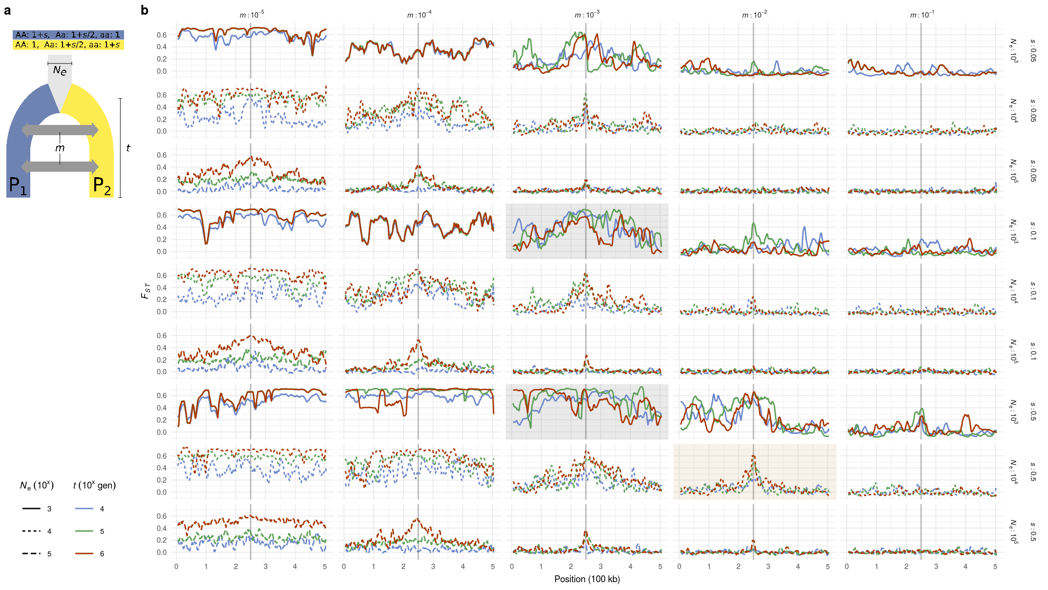
10 Supplementary Figure 05

10.1 Summary

This is the accessory documentation of Supplementary Figure 05.

The Figure can be recreated by running the R script S05.R:

cd $WORK/3_figures/F_scripts

Rscript --vanilla S05.R
rm Rplots.pdf

10.2 Details of S05.R

In the following, the individual steps of the R script are documented. Is an executable R script that depends on a variety of image manipulation and data managing packages.

It Furthermore depends on the R scripts S05.functions.R and S05.facet_reverse.R (both located under $WORK/0_data/0_scripts).

In the start-up section the prefix and the directory of the simulation results is defined.

library(tidyverse)
library(grid)
library(gridSVG)
library(grImport2)

name <- 'simulated_'
fst_base <- '../../2_output/10_simulation/fst/'
fun_script <- '../../0_data/0_scripts/S05.functions.R'
rev_script <- '../../0_data/0_scripts/S05.facet_reverse.R'
source(fun_script)
source(rev_script)

The simulation results are collected and the function read_data() is generated to later import the simulation results. This function reads in the data, extracts the parameter settings of the individual runs given in the file name and stores them with the data.

files <- dir(fst_base,pattern = 'weir.fst$')

read_data <- function(in_file){read_delim(str_c(fst_base,in_file),delim = '\t') %>%
    mutate(POS = (BIN_START+BIN_END)/2,
           run = str_extract(string = in_file,"n.*.wi") %>%
             str_remove(.,'n.') %>%
             str_remove(.,'.wi'),
           run2 = run) %>%
    separate(run2,into = c('ext','rec','italic(N)[e]','italic(s)','italic(m)','divt','dom'),
             convert = TRUE,sep = '_') %>% 
    mutate(`italic(N)[e]` = log10(`italic(N)[e]`) %>% str_c('10^',.,''),
           `italic(m)` = log10(`italic(m)`) %>% str_c('10^',.,''))
  }

The simulation results are imported and the factor levels of some parameters are reordered.

data <- purrr::map(files,read_data) %>% bind_rows()
lv <- data$`italic(m)` %>% as.factor() %>% levels()
data$`italic(m)` <- factor(data$`italic(m)`,levels = rev(lv))
yl <- expression(italic('F'[ST]))

A helper data frame is created to highlight the background of specific simulation scenarios.

bg <- tibble(`italic(s)` = c("0.1","0.5","0.5"),
             `italic(N)[e]` = c(rep("10^3",2),"10^4"),
             `italic(m)` = c(rep("10^-3",2),"10^-2"),
             case = letters[c(1,1,2)],col = c(NA,NA,'black'))

The simulation results are plotted.

p <- ggplot()+
  # indicate the selected locus
  geom_vline(xintercept = 2.5,col=rgb(0,0,0,.25))+
  #background highlighting
  geom_rect(inherit.aes = FALSE,
            data=bg,aes(fill=case),
            xmin=-Inf,xmax=Inf,ymin=-Inf,ymax=Inf,
            col=NA)+
  # plot the simulation results
  geom_line(data = data,aes(x=POS/100000,
                y=WEIGHTED_FST,
                col=factor(log10(divt)),
                linetype=factor(`italic(N)[e]`)))+
  # define color palette
  scale_color_manual(name = expression(italic(t)~(10^x~gen)),
                     values = c(scico::scico(n = 7,
                                             palette = 'tofino')[c(2,6)],
                                RColorBrewer::brewer.pal(5,'Oranges')[5]))+
  # define highlighting colors
  scale_fill_manual(values = c(rgb(.2,.2,.2,.1),rgb(.7,.5,.2,.1)),guide=FALSE)+
  # define line types
  scale_linetype(name = expression(italic(N)[e]~(10^x)),labels = 3:5)+
  # X & Y labels
  scale_x_continuous('Position (100 kb)')+
  scale_y_continuous(name = yl)+
  # order scenarios within grid depending on parameter settings
  facet_reverse(rows = vars(`italic(s)`,`italic(N)[e]`),
             cols  = vars(`italic(m)`),as.col_table = FALSE,
            labeller = label_both_parsed)+
  # general plot theme
  theme_minimal(base_size = 7)

The side annotation of the plot is created by extracting the plot legend and importing the basic scheme of the demographic history modeled.

# extracting the legend
leg <- (p+guides(color = guide_legend(direction = 'vertical'),
                  linetype = guide_legend(direction = 'vertical'))+
          theme(legend.position = 'bottom')) %>% 
  cowplot::get_legend()
# importing the model scheme
mod <- gTree(children=gList(pictureGrob(readPicture("../../0_data/0_img/model-cairo.svg"))))
# putting together the side annotation
side <- cowplot::plot_grid(mod,NULL,leg,ncol=1,rel_heights = c(1,1,.6))

Using plot_grid() form the cowplot package, the figure is put together.

S05 <- cowplot::plot_grid(side,(p + theme(legend.position = 'none')),
                          nrow = 1,rel_widths = c(.15,1),labels = c('a','b'),label_size = 10)

It is then exported using ggsave().

ggsave(plot = S05,filename = '../output/S05.pdf',width = 284,height = 160,units = 'mm',device = cairo_pdf)

---