15 Supplementary Figure 10
15.1 Summary
This is the accessory documentation of Supplementary Figure 10.
The Figure can be recreated by running the R script S10.R:
cd $WORK/3_figures/F_scripts

Rscript --vanilla S10.R
rm Rplots.pdf
15.2 Details of S10.R
In the following, the individual steps of the R script are documented. Is an executable R script that depends on a variety of image manipulation and data managing packages.
library(RColorBrewer)
library(tidyverse)
library(cowplot)
library(gridExtra)
library(gtable)
library(grid)
library(colorspace)
library(gdata)
library(hrbrthemes)
theme_set(theme_minimal())
The hamlet LG color palette is generated.
clr_LGs <- c(rgb(10,36,106,max=255),rgb(10,48,118,max=255),rgb(10,60,129,max=255),
             rgb(10,72,141,max=255),rgb(11,84,153,max=255),rgb(11,96,164,max=255),
             rgb(11,108,176,max=255),rgb(11,120,187,max=255),rgb(11,132,199,max=255),
             rgb(37,131,174,max=255),rgb(64,130,149,max=255),rgb(90,129,124,max=255),
             rgb(117,129,100,max=255),rgb(143,128,75,max=255),rgb(169,127,50,max=255),
             rgb(196,126,25,max=255),rgb(222,125,0,max=255),rgb(213,109,0,max=255),
             rgb(205,94,0,max=255),rgb(196,78,0,max=255),rgb(188,63,0,max=255),
             rgb(179,47,0,max=255),rgb(170,31,0,max=255),rgb(162,16,0,max=255),
             rgb(153,0,0,max=255),rgb(.5,.5,.5))
15.2.1 Reading in Data
Then,the extent of the individual LGs in loaded.
seqStart <- read.csv('../../0_data/0_resources/seqSTART.csv',sep='\t')
karyo <- read.csv('../../0_data/0_resources/F2.karyo.txt',sep='\t') %>%
  mutate(GSTART=lag(cumsum(END),n = 1,default = 0),
         GEND=GSTART+END,GROUP=rep(letters[1:2],12)) %>%
  select(CHROM,GSTART,GEND,GROUP)
The data for the two Parents from the linkage cross are loaded individually and combined with the genomic positions retrieved from the mapping of the RAD tags.
Parent 1: First the linkage data is loaded from the excel sheet. The columns are renamed, the LGs transformed from Roman tho Arabic numbers and the RAG tag IDs are reformatted.
hypo_map1.9 <- read.xls ("../../0_data/0_resources/Hypoplectrus_nigricans_Linkage_map.xls", sheet = 1, header = TRUE)[,1:3]
names(hypo_map1.9)<-c("Loci","LG","cM")
hypo_map1.9$LG <- as.numeric(as.roman(as.character(hypo_map1.9$LG)))
hypo_map1.9$Loci <- gsub("_ab?","",hypo_map1.9$Loci)
The increase in cM is calculated for each locus (cMn - cMn-1). This is done within each LG on its own.
cM1 <- hypo_map1.9 %>% group_by(LG)  %>%
  mutate(abs_cM = cM-lag(cM,default = 0)) %>%
  ungroup() %>%select(Loci,cM,abs_cM)
Then the mapping positions of the RAD tags are loaded. The order of the LGs is set and the genomic bin position of the RAD tag is calculated
(The bin is the stretch between the current locus and the previous one. The position and extend of the bin are later combined with the increase of cM between the two loci.)
bp1 <- read.csv('../../1-output/10_recLandscape/MAP1Mb.txt',
                  sep='\t',head=F,col.names = c("Loci","LG",'bp'))
bp1$LG <- factor(as.character(bp1$LG),levels=as.character(seqStart$LG))
bp1 <- bp1 %>%
  arrange(LG,bp) %>% group_by(LG) %>%
  mutate(bin_bp = lag(bp,default = 0)+(bp-lag(bp,default = 0))/2,
         strech = bp-lag(bp,default = 0))
The linkage and mapping data are merged, the position by LG is transformed to genomic position and the linkage density (as cM/Mp) is calculated. Also, a parent ID column is added.
data1 <- merge(merge(bp1,cM1,by='Loci'),seqStart,by='LG') %>% arrange(LG,bin_bp) %>%
  mutate(POS = genomicStart+bin_bp,den_cM = abs_cM/strech*1000000) %>%
  filter(grepl('LG',LG)) %>%
  mutate(Parent="Parent 1")
The data for parent two is loaded in the same way as for parent one.
hypo_map2.9 <- read.xls ("../../0_data/0_resources/Hypoplectrus_nigricans_Linkage_map.xls", sheet = 2, header = TRUE)[,1:3]
names(hypo_map2.9)<-c("Loci","LG","cM")
hypo_map2.9$LG <- as.numeric(as.roman(as.character(hypo_map2.9$LG)))
hypo_map2.9$Loci <- gsub("_ab","",as.character(hypo_map2.9$Loci)) %>% as.integer()

cM2 <- hypo_map2.9 %>% group_by(LG)  %>%
  mutate(abs_cM = cM-lag(cM,default = 0)) %>%
  ungroup() %>%select(Loci,cM,abs_cM)

bp2 <- read.csv('../../1-output/10_recLandscape/MAP2Mb.txt',
                sep='\t',head=F,col.names = c("Loci","LG",'bp'))
bp2$LG <- factor(as.character(bp2$LG),levels=as.character(seqStart$LG))
bp2 <- bp2 %>%
  arrange(LG,bp) %>% group_by(LG) %>%
  mutate(bin_bp = lag(bp,default = 0)+(bp-lag(bp,default = 0))/2,strech = bp-lag(bp,default = 0))

data2 <- merge(merge(bp2,cM2,by='Loci'),seqStart,by='LG') %>% arrange(LG,bin_bp) %>%
  mutate(POS = genomicStart+bin_bp,den_cM = abs_cM/strech*1000000) %>%
  filter(grepl('LG',LG)) %>%
  mutate(Parent="Parent 2")
The data sets of the two parents are combined.
dataMERGE <- rbind(data1,data2)
dataMERGE$LG <- drop.levels(dataMERGE$LG)
15.2.2 Subfigure S10 a
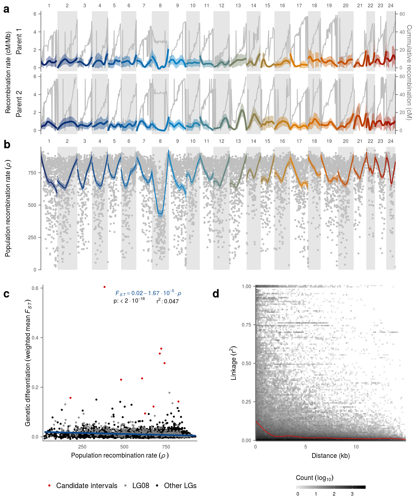
Colors are set for the plot (background color for the LGs, raw cM data, secondary y axis & labels) Also the ratio of primary Y axis and secondary Y axis as well as the Y axis labels are set. Also the overall them of the figure is pre-defined.
lgclr <- rgb(.9,.9,.9)
annoclr <- rgb(.4,.4,.4)
secclr <- rgb(.75,.75,.75)
secclrLAB <- rgb(.45,.45,.45)
secScale <- 10
YL1 <- "Recombination rate (cM/Mb)"
YL2 <- "Cummulative recombination (cM)"

theme_gw <- theme(plot.margin = unit(c(2,5,2,0),'pt'),
                  panel.grid = element_blank(),
                  panel.spacing.y = unit(3,'pt'),
                  legend.position = 'none',
                  axis.title.x = element_blank(),
                  axis.ticks.y = element_line(color = annoclr),
                  axis.line.y =  element_line(color = annoclr),
                  axis.text.x = element_text(size=6),
                  axis.text.y = element_text(margin = unit(c(0,3,0,0),'pt'),size=6),
                  axis.title.y = element_text(vjust = -1,size=8),
                  axis.title.y.right = element_text(color=secclrLAB,size=8),
                  axis.text.y.right = element_text(color=secclrLAB,size=6),
                  strip.background = element_blank(),
                  strip.placement = "outside")
Then sub figure a is plotted:
S10a <- ggplot()+
  # background shading for LGs
  geom_rect(inherit.aes = F,data=karyo,aes(xmin=GSTART,xmax=GEND,
                                           ymin=-Inf,ymax=Inf,fill=GROUP))+
  # adding raw cM data
  geom_line(data=dataMERGE,aes(x=POS,y=`cM`/secScale),col=secclr)+
  # adding a smoothed fith of the recombination density
  geom_smooth(data=dataMERGE,aes(x=POS,y=`abs_cM`,col=LG,fill=LG),
              size=1,method = 'loess',span=0.7,se=T)+
  # separate the data by parent
  facet_grid(Parent~.,switch = "y")+
  # set color palettes
  scale_fill_manual(values = c(NA,lgclr,alpha(clr_LGs,.3)),guide=F)+
  scale_color_manual(values=clr_LGs)+
  # format x and y axis
  scale_x_continuous(expand = c(0,0),
                     breaks = (karyo$GSTART+karyo$GEND)/2,
                     labels = 1:24,position = "top")+
  scale_y_continuous(name=YL1,limits = c(-.1,6),
                     sec.axis = sec_axis(~.*secScale,name=YL2))+
  # plot layout theme
  theme_gw
15.2.3 Subfigure S10 b
Sub figure b and c depend on the fasteprr output and on the respective F[ST] values of the analyzed windows:
data_rho <- read.delim(gzfile('../../2_output/08_popGen/12_fasteprr/step4/fasteprr.all.rho.txt.gz'),stringsAsFactors = FALSE) %>%
  mutate(POS = (BIN_START+BIN_END)/2,
         LGBIN = str_c(CHROM,BIN_START))

data_fst <-  read.delim(gzfile('../../2_output/08_popGen/05_fst/fst.global.nonoverlap.50kb.windowed.weir.fst.gz'),
                        stringsAsFactors = FALSE) %>%
  mutate(LGBIN = str_c(CHROM,BIN_START)) %>%
  select(LGBIN,WEIGHTED_FST)

data_rho_gw <- left_join(data_rho,karyo,by='CHROM') %>% mutate(GPOS=POS+GSTART,group='')
Sub figure b is plotted:
S10b <- ggplot()+
  geom_rect(inherit.aes = F,data=karyo,
            aes(xmin = GSTART,xmax = GEND,
                ymin = -Inf,ymax = Inf,fill = GROUP))+
  geom_point(data=data_rho_gw,aes(x=GPOS,y=RHO),col=secclr,size=.5)+
  geom_smooth(data=data_rho_gw,aes(x=GPOS,y=RHO,color=CHROM,fill=CHROM),lwd=.5)+
  scale_fill_manual(values = c(NA,lgclr,alpha(clr_LGs,.3)),guide=F)+
  scale_color_manual(values=clr_LGs)+
  scale_x_continuous( name = '', expand = c(0,0),
                      breaks = (karyo$GSTART + karyo$GEND) / 2,
                      labels = 1:24, position = "top")+
  facet_grid(group~.,switch = "y")+
  scale_y_continuous(name=expression(Population~recombination~rate~(italic("\u03C1"))),
                     limits = c(0,950),expand = c(0,0))+
  theme_gw
15.2.4 Subfigure S10 c
To classify the fasteprr results as belonging to either LG08, the candidate gene regions or to the standard region of the genome the outl_window function is defined and applied to the combined data.
BINWDTH <- 50000
outl_window <- function(LGBIN){
  lg = str_sub(LGBIN, 1, 4)
  bin = str_sub(LGBIN, 5) %>% as.numeric()

  if (lg == "LG09") {
    out <- c("Other LGs","Candidate intervals")[between(x = bin,left = 17821000,right = 17930000-BINWDTH)+1]
    return(out)
  } else if (lg == "LG12") {
    out <- c("Other LGs","Candidate intervals")[(between(x = bin,left = 20085000,right = 20355000-BINWDTH) | between(x = bin,left = 22150000,right = 22290000-BINWDTH))+1]
    return(out)
  } else if (lg == "LG17") {
    out <- c("Other LGs","Candidate intervals")[between(x = bin,left = 22505000,right = 22660000-BINWDTH)+1]
    return(out)
  }
  return("Other LGs")
}

data_both <- full_join(data_rho,data_fst,by='LGBIN') %>% rowwise() %>%
  mutate(gr = ifelse(CHROM=="LG08","LG08",outl_window(LGBIN)))
The regression of the dependence of divergence on recombination rate is modeled and r^2, p-value, slope and intercept are exported.
mod <- lm(data_both$WEIGHTED_FST~data_both$RHO)
sumMOD <- summary(mod)
modA <- round(mod$coefficients[[1]],3)
modB <- round(mod$coefficients[[2]],7)
The labels of sub figure 10 are set.
modclr <- clr_LGs[4]
an1 <- expression("p: < 2"%.%"10"^-16)
an2 <- paste0('r^2:',round(sumMOD$adj.r.squared,3))
an3 <- paste0("italic(F[ST]) == ",modA,modB*10^5," %.% 10^-5"," %.% italic(\u03C1)")
Sub figure c is plotted:
S10c <- ggplot(data_both,aes(x=RHO,y=WEIGHTED_FST))+
  geom_point(data=(data_both %>% filter(gr=="Other LGs")),aes(color=gr),size=.5)+
  geom_point(data=(data_both %>% filter(gr=="LG08")),aes(color=gr),size=.5)+
  geom_point(data=(data_both %>% filter(gr=="Candidate intervals")),aes(color=gr),size=.5)+
  geom_smooth(method='lm',
              col=modclr,fill=rgb(.9,.9,.9,.001))+
  annotate(geom = 'text',x=c(795)-150,y=c(.58),label=an3,size=2.5,parse=TRUE,col=modclr)+
  annotate(geom = 'text',x=c(745)-215,y=c(.55),label=an1,size=2.5)+
  annotate(geom = 'text',x=c(865)-105,y=c(.55),label=c(an2),parse=TRUE,size=2.5)+
  scale_x_continuous(name=expression(Population~recombination~rate~(italic("\u03C1"))),
                     expand = c(.01,.01))+
  scale_y_continuous(name=expression(Genetic~differentiation~(weighted~mean~italic(F[ST]))),
                     expand = c(.005,.005))+
  scale_color_manual(name = 'Group',values = c('#d40606',rgb(.5,.5,.5,.8),'black'))+
  theme_gw+theme(plot.background = element_blank(),
                 panel.background  = element_blank(),
                 panel.grid=element_blank(),
                 panel.border = element_blank(),
                 plot.margin = unit(c(0,15,0,25),'pt'),
                 axis.line.x =  element_line(color = annoclr),
                 axis.text.x = element_text(size=6),
                 axis.title.x = element_text(size=8),
                 legend.position = 'bottom',
                 legend.title = element_blank())
15.2.5 Subfigure S10 d
Loading the linkage decay data:
decay_path <- '../../2_output/08_popGen/07_LD/decay/'
files_d <- dir(path = decay_path,pattern = 'ld.gz')
read_r2 <- function(file){read_delim(file = str_c(decay_path,file),delim = '\t')}
data_d <- files_d %>% purrr::map(.,read_r2) %>% bind_rows()
Sub figure d is plotted:
S10d <- ggplot(data=data_d,aes(x=(POS2-POS1)/1000,y=`R^2`))+
    geom_hex(bins = 100,aes(fill=log10(..count..))) +
    geom_smooth(col='red',se=FALSE,size=.3,
                method = 'gam', formula = y ~ s(x, bs = "cs"))+
    scale_fill_gradient(name = expression(Count~(log[10])),
                        low = rgb(.9,.9,.9), high = "black")+
    guides(fill=guide_colorbar(direction = 'horizontal',title.position = 'top'))+
    scale_x_continuous(name = "Distance (kb)",expand = c(0,0))+
    scale_y_continuous(name = expression(Linkage~(r^2)),
                       expand = c(0.002,0.002))+
    theme_gw+
    theme(plot.background = element_blank(),
          panel.background  = element_blank(),
          panel.grid = element_blank(),
          panel.border = element_blank(),
          plot.margin = unit(c(0,15,0,25),'pt'),
          axis.line =  element_line(color = annoclr),
          axis.text = element_text(size=6),
          axis.title.x = element_text(size=8),
          axis.title.y = element_text(size=8,vjust = 1),
          legend.title = element_text(size=8),
          legend.text = element_text(size=6),
          legend.key.height = unit(4,'pt'),
          legend.position = 'bottom')
Finally, supplementary figure 10 is assembled.
S10ab <- plot_grid(S10a,S10b,ncol = 1,align = 'v',labels = c('a','b'))
S10cd <- plot_grid(S10c,S10d,nrow = 1,labels = c('c','d'),align = 'h')
S10 <- plot_grid(S10ab,NULL,S10cd,ncol = 1,rel_heights = c(1,.05,.8))
This is then exported using ggsave().
ggsave(plot = S10,filename = '../output/S10.pdf',width = 183,height = 220,units = 'mm',device = cairo_pdf)