Rayshader + Marmap
Combining the bathymethric import function of marmap with the beauty of rayshader
What: Creating the obligatory rotating gif
Motivation
I’m a big fan of maps in general and I love using R to work with spatial data. Because of this, I have been quite excited by the development of the great rayshader package by Taylor Morgan-Wall (Morgan-Wall 2019).
Over the last months, great examples of stunning 3d models have mushroomed (#rayshader), yet most of these depict terrestrial scenes. I guess this might be due to the good availability of data from DEMs (Digital elevation models) compared to bathymetric data sets.
As I have been using another great package - marmap (Pante 2013) - to plot bathymetric map for quite some time now, I thought these two packages might complement each other quite well.
So below, I want to give a small presentation how rayshader can be used in combination with marmap to produce some nice 3D-models of marine landscapes. A small caveat is that the NOAA data sets importable by marmap are rather of coarse resolution, so this works best on a large scale.
Packages
Besides the two packages of focus (rayshader and marmap), I work within the tidyverse and I need the magic package to modify some overlay images and create the obligatory rotating gif at the end.
library(rayshader)
library(marmap)
library(tidyverse)
library(magick)
Helper functions
To easily import and use satellite images as overlay I follow a nice tutorial by Will Bishop and import functions from his accompanying repository.
source('rayshader-demo/R/image-size.R')
source('rayshader-demo/R/map-image-api.R')
source('rayshader-demo/R/find-image-coordinates.R')
source('rayshader-demo/R/rayshader-gif.R')
I also create two small functions to ease the introduction of labels hovering over the 3D model. These are built around the functions provided by Will Bishop.
get_label <- function(label, long, lat, image_size,bbox){
  label <- list(text = label)
  label$pos <- find_image_coordinates(
    long = long, lat = lat, bbox = bbox,
    image_width = image_size$width,
    image_height = image_size$height)
  label$pos$y <- image_size$height - label$pos$y
  label$pos$x <- image_size$width - label$pos$x
  return(label)
}

render_lab <- function(rb,label){
  render_label(rb, x = label$pos$x, y = label$pos$y, z = 3500,
               zscale = zz, text = label$text, textsize = 1, linewidth = .8)
}
The last function we need is one that will flip the bathymetric data set because for some reason it gets mirrored when used with rayshader.
rev_bat <- function(bat){
  x <- bat %>% dim() %>% .[1]
  bat[x:1,]}
Setup
The first thing we need to do is to define the bounding box (the
extent) of the region we want to model. For this we define a list()
containing the minimum & maximum of longitude and latitude. Here, I
download the entire greater Caribbean.
bbox <- list(
  p1 = list(long = -102, lat = 5),
  p2 = list(long = -60, lat = 32)
)
Now, we use marmap to import the elevation and bathymetric data for the region of interest.
bat <- marmap::getNOAA.bathy(bbox$p1$long, bbox$p2$long,
                     bbox$p1$lat, bbox$p2$lat, resolution = 3)
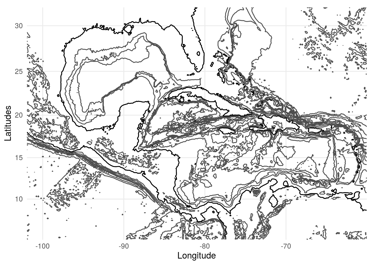
Using ggplot2 we can do a quick check of the extent.
bat %>%
  autoplot() +
  scale_x_continuous('Longitude', expand = c(0, 0))+
  scale_y_continuous('Latitudes', expand = c(0, 0))+
  theme_minimal()
For the use with rayshader we flip the data set and define the level of vertical exaggeration.
rb <- bat %>% rev_bat()
zz <- 500
Than we create the rayshader- and the ambient-shadow layer of the model.
rb_shadow = ray_shade(rb,zscale=zz,lambert=TRUE)
rb_amb = ambient_shade(rb,zscale=zz)
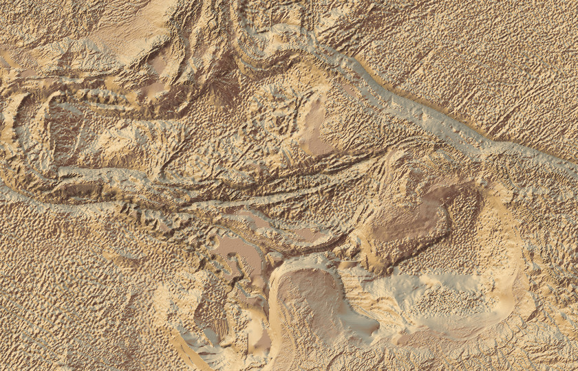
Now we can take a first look at the model.
rb %>%
  sphere_shade(texture = "desert") %>%
  add_shadow(rb_shadow, max_darken = 0.5) %>%
  add_shadow(rb_amb, max_darken = 0.5) %>%
  plot_map()
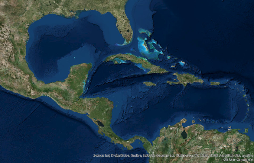
Overlay images
Now, we will create some overlay images following the example from Will Bishop. For this we need to know the size of the imported data set since the overlay image and the 3D-model need to match.
wdth <- bat %>% as.matrix() %>% dim()
image_size <- define_image_size(bbox, major_dim = wdth[1])
With this information we can download an overlay image spanning the previously defined bounding box with the correct resolution to match the data set.
overlay_file <- "sf-map.png"
get_arcgis_map_image(bbox, map_type = "World_Imagery", file = overlay_file,
                     width = image_size$width, height = image_size$height,
                     sr_bbox = 4326)
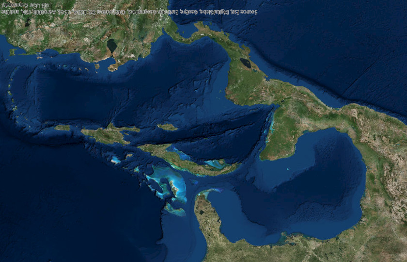
For some reason we need to rotate it by 180° for the use with rayshader. We can do this using the magic package.
image_read(overlay_file) %>%
  image_rotate(.,180) %>%
  image_write(str_replace(overlay_file,'.png','_3d.png'))
overlay_img <- png::readPNG(overlay_file)
overlay_3d <- png::readPNG(str_replace(overlay_file,'.png','_3d.png'))
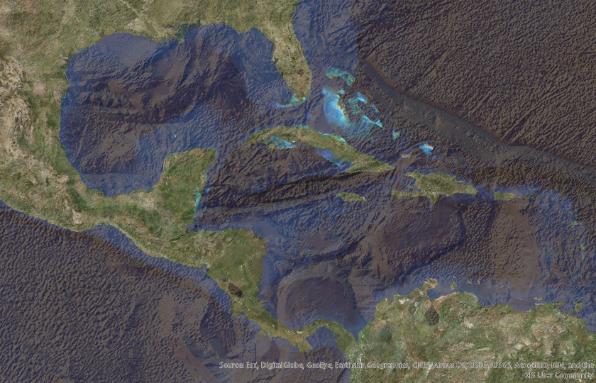
We can now add this image as an overlay layer for the 3D-model.
rb %>%
  sphere_shade(texture = "desert") %>%
  add_shadow(rb_shadow, max_darken = 0.5) %>%
  add_shadow(rb_amb, max_darken = 0.5) %>%
  add_overlay(overlay_img, alphalayer = 0.85) %>%
  plot_map()
Labels
We create labels for points within the bounding box. Here, I want to label the research station of the Smithsonian in Panama as well as Havana and Cancun.
stri <- get_label("STRI",long = -82.256951,lat = 9.351997, image_size, bbox)
havana <- get_label('Havana', -82.391467, 23.069702, image_size, bbox)
cancun <- get_label('Cancun', -86.851510, 21.135076, image_size, bbox)
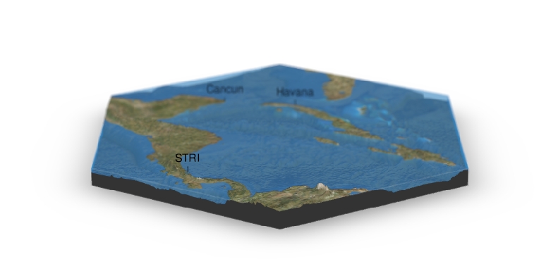
3D-model
Finally, it is time to put all the pieces together and create the 3D-model.
Base model
rb %>%
  sphere_shade(texture = "desert")  %>%
  add_shadow(rb_shadow, max_darken = 0.5) %>%
  add_shadow(rb_amb, max_darken = 0.5) %>%
  add_overlay(overlay_3d, alphalayer = 0.8) %>%
  plot_3d(rb,
          zscale = zz,
          fov = 30,
          theta=210, # <-->
          phi=21,    # |
          windowsize = c(800,400),
          zoom = .3,
          water=TRUE,
          waterdepth = 0,
          wateralpha = 0.6,
          watercolor = "#3182BD",
          waterlinecolor = "white",
          waterlinealpha = 0.1,
          baseshape = 'hex')
# Add labels
render_lab(rb = rb,label = stri)
render_lab(rb = rb,label = cancun)
render_lab(rb = rb,label = havana)
# create snapshot
render_depth(focus = 0.45, focallength = 25)
When running this within Rstudio this will create a nice interactive 3D-model, but here you can only look at the snapshot - bummer!

Move it
To still provide you with an idea of the full model, we’ll create an animated gif from a series of snapshots. At this point I deviate from the nice concise example from Will Bishop since I want to make use of the illusion of a limited field of depth provided by the accessory package rayfocus.
First, we need to decide on the number of frames for the animation. Then we will create a new theta value for each frame to complete a full rotation of 360° during the animation.
n_frames <- 180
# Frame transition variables
thetavalues <- seq(210,-150, length.out = n_frames)
Then, we loop over the frames and export each one as single png file.
generate .png frame images
img_frames <- paste0("drain", seq_len(n_frames), ".png")
for (i in seq_len(n_frames)) {
  # message to follow the progress along the loop
  message(paste(" - image", i, "of", n_frames))
  # create the model
  rb %>%
    sphere_shade(texture = "desert")  %>%
    add_shadow(rb_shadow, max_darken = 0.5) %>%
    add_shadow(rb_amb, max_darken = 0.5) %>%
    add_overlay(overlay_3d, alphalayer = 0.8) %>%
    plot_3d(rb,
            zscale=zz,
            fov = 30,
            theta=thetavalues[i], # <-->
            phi=21,    # |
            windowsize=c(800,400),
            zoom = .3,
            water=TRUE,
             waterdepth = 0,
            wateralpha = 0.6,
            watercolor = "#3182BD",
            waterlinecolor = "white",
            waterlinealpha = 0.1,
            baseshape = 'hex')
  # add labels
  render_lab(rb = rb,label = stri)
  render_lab(rb = rb,label = cancun)
  render_lab(rb = rb,label = havana)
  # take snapshot
  render_depth(filename = img_frames[i],
               focus=0.45,
               focallength = 25)
  # erase model
  rgl::clear3d()
}
Finally, we again use the magic package to fuse all the frames into a single gif file to get our spinning model.
magick::image_write_gif(magick::image_read(img_frames),
                        path = "ray_caribbean.gif",
                        delay = 10/n_frames)
References
Morgan-Wall, Tyler. 2019. Rayshader: Create and Visualize Hillshaded Maps from Elevation Matrices. https://github.com/tylermorganwall/rayshader.
Pante, Benoit, Eric AND Simon-Bouhet. 2013. “Marmap: A Package for Importing, Plotting and Analyzing Bathymetric and Topographic Data in R.” PLOS ONE 8 (9). Public Library of Science: 1–4. https://doi.org/10.1371/journal.pone.0073051.