Recolor svg files

Load svg files

The hypoimg package provides tools read external svg files into R to use for plot annotation. (The svg needs to be a cairo svg - to transform your svg into this format use the rsvg package)

rsvg::rsvg_svg("image.svg","image.c.svg")

library(tidyverse)
library(grImport2)
library(grid)
library(gridSVG)

svg_file <- system.file("extdata", "logo.c.svg", package = "hypoimg")
svg <- hypo_read_svg(svg_file)

ggplot(tibble(x=rnorm(100),y=rnorm(100)))+
  annotation_custom(svg)+
  geom_point(aes(x=x,y=y),
             color="#AA1F00")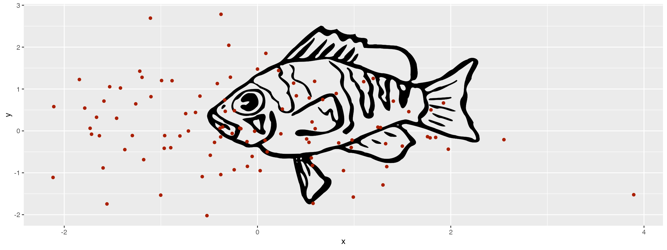

Recolor single layer

Individual layers of the image can be recolored using the hypo_recolor_svg() function:

svg_new <- hypo_recolor_svg(svg, layer = 1, color = "#2B5B99")
ggplot()+
  annotation_custom(svg_new)

This can be used to create a table of color variants:

n = 9
tab <- hypo_recolor_grob_table(svg,
                          LETTERS[1:n],
                          scico::scico(n, palette = 'lapaz'),
                          angle = rnorm(n)*60,
                          layer = 1)

ggplot(tibble(x=1:2),aes(x=x,y=x))+
  geom_hypo_grob(data=tab,
                 aes(grob=grob,x=x,y=y,
                     angle=angle),
                 width=.6)+
  facet_wrap(grp~.,ncol = 3)+
  theme(text=element_blank(),
        axis.ticks = element_blank())

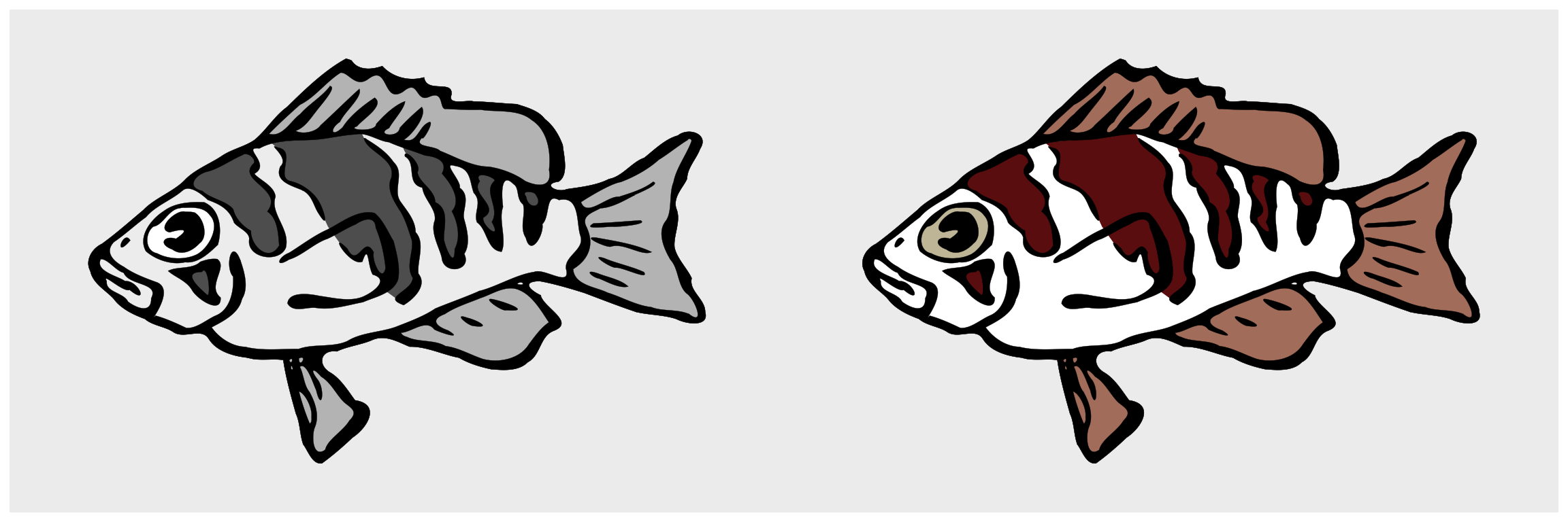
Finally, hypo_recolor_svg() can be applied multiple times to recolor several layers:

svg_file_2 <- system.file("extdata", "logo2.c.svg", package = "hypoimg")
svg_2 <- hypo_read_svg(svg_file_2)

clr <- scico::scico(25)
ggplot()+
  annotation_custom(svg_2,xmax = .5)+
  annotation_custom(svg_2 %>%
                      hypo_recolor_svg(.,layer = 1,clr[1]) %>%
                      hypo_recolor_svg(.,layer = 2,clr[8]) %>%
                      hypo_recolor_svg(.,layer = 3,clr[16]) %>%
                      hypo_recolor_svg(.,layer = 4,clr[24]),
                    xmin = .5)

---