Baboons on the move
Following the collective movement behavior of a pack of olive baboons
What: Animate animal movement data from movebank.org in R.
Motivation
I recently got a copy of Where the Animals Go by Uberti and Cheshire (2018). This cool book is pure eye candy for anyone who is interested in maps and/or animals and I highly recommend to have a look at it. It is filled with extremely well done visualizations of animal movement data and accompanying stories about the protagonists and the researchers studying them.
Many of the maps within the book bring the animal to life and really give a feel for the dynamics of their movements - yet it is a print product and therefore static. So, since Uberti and Cheshire provide their data source - Scientist who make their tagging data publicly available (open data! :D) - I just could not resist to actually look at the movement of one of the stories:
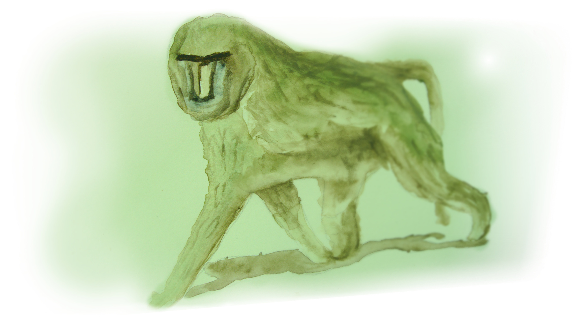
I chose the story about the collective movement of a group of Olive baboons (Papio anubis, p. 48-51) mostly because the detail panels of this piece already look like a Flip book which made animating this data set seem like a natural choice.
This story is based on a publication by Strandburg-Peshkin et al. (2015), who used GPS collars to collect a data set that is of incredibly fine scale both in terms of spatial as well as temporal resolution (1 GPS position/s). Much to the authors credit, they made the data set easily available on the data repository movebank (Crofoot, Kays, and Wikelski 2015).
It was therefore fairly straight forward to dive into the data and explore the baboon story in some more detail:
Packages
To create the baboon movement animation, I relied on a whole set of R packages to tackle the different aspects of this project:
Mapping tools
By now, basically all my R code relies on the tidyverse, so this not exactly mapping specific (although the mapping is done with ggplot2). The rest of these packages are needed to work with or to plot spatial data.
library(tidyverse)
library(ggmap)
library(sf)
library(smoothr)
library(raster)
Mapping data
For this project we also use some external spatial data sets to provide context for the movement data. The package osmdata is a convenient way to access open street map data - here we will import the rivers Ewaso Ng’iro and Nanyuki. We will use the package rnaturalearth to access the outline of Kenya.
library(osmdata)
library(rnaturalearth)
Mapping annotations and layout
Besides the spatial data, the animation is going to include some graphical annotations. We’ll use ggspatial to add a scale bar and a compass and extrafont to use non-standard fonts to create a look more like that of Uberti and Cheshire.
library(ggspatial)
library(extrafont)
Animation
Finally, to get some action, we’ll use gganimate.
library(gganimate)
Preparation
Before we start with the data wrangling, we set some configurations:
- we adjust the animation output formats
- we set the color palette for the baboons
- we write a small function to crop spatial data with our bounding box
options(gganimate.dev_args = list(width = 450, height = 180))

clr <- c(m = RColorBrewer::brewer.pal(5,'Blues')[4],
         f = RColorBrewer::brewer.pal(5,'Reds')[4])

crp <- function(poly){
  st_intersection(poly,st_set_crs(st_as_sf(as(raster::extent(36.922, 36.929,
                                                             0.35, 0.353),
                                              "SpatialPolygons")), st_crs(poly)))
}
Import and filter movement data
Of course, the most important data here ist the baboon movement data from Crofoot, Kays, and Wikelski (2015) which we download from movebank.
The data set contains two files - one with the actual GPS positions (collective_movement.csv.gz) and one with the metadata (baboon id, sex, etc; collective_movement-reference.csv.gz).
For readability and storage reasons I renamed and gzipped the original files, otherwise the data files are not modified.
data <- read_csv('collective_movement.csv.gz')
meta <- read_csv('collective_movement-reference.csv.gz') %>%
  dplyr::select(`animal-id`,`animal-life-stage`,`animal-mass`,`animal-sex`) %>%
  setNames(., nm = c('individual-local-identifier', 'stage','mass', 'sex'))
The detail panels of Uberti and Cheshire (p. 50, 51) only show the small part of the data that was collected on the first of August between 08:00 and 08:30 (EAT time zone). So we also subset the data set to this time frame. We also gather the weight of the largest baboon that we will need later for scaling.
strt_time <-lubridate::as_datetime("2012-08-01 05:00:00 UTC")
end_time <-lubridate::as_datetime("2012-08-01 05:30:00 UTC")

data_track <- data %>%
  filter(between(timestamp,strt_time,end_time)) %>%
  left_join(., meta) %>%
  setNames(., nm = c('timestamp', 'long', 'lat', 'id', 'stage', 'mass', 'sex'))

max_mass <- max(data_track$mass)
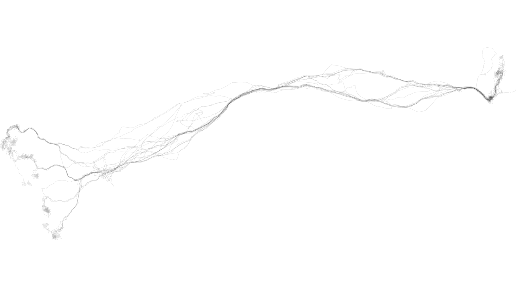
Time to inspect our subset and to have a first look if we see the same pattern as in the book.
ggplot()+
  geom_path(inherit.aes = FALSE, data = data_track %>% dplyr::select(-timestamp),
                       aes(x = long, y = lat,
                           color = sex, group = id),
                       color = rgb(0,0,0,.1),size=.2)+
  coord_sf() +
  scale_y_continuous(expand = c(0,0))+
  scale_x_continuous(expand = c(0,0))+
  scale_color_manual(values = alpha(clr, .5), guide=FALSE)+
  theme_void()+
  theme(legend.position = 'none',
        line = element_line(color=rgb(0,0,0,0), size = .1, linetype = 1, lineend = 'round'),
        plot.title = element_text(hjust = 0.5,face = 'italic',family = 'Georgia',margin = margin(t = 10, b = -20)))
Load rivers from open street map
Now that we are done with the movement data, let’s tackle the data for mapping context. Therefore, we first define the bounding box within which we are going to collect background data and create the query to access open street map data.
bb <- c(36.922, 0.35, 36.929,  0.353)
bb_tib <- tibble(x1=bb[1],x2=bb[3],y1=bb[2],y2=bb[4])

q_sf <- opq(bbox = bb) %>%
  add_osm_feature(key = 'name') %>%
  osmdata_sf ()
Then, we extract the rivers from the open street map data, smooth it (because of its relatively coarse resolution) and crop it with the bounding box.
rivers <- q_sf$osm_lines[ which(q_sf$osm_lines$waterway == 'river'), ] %>% crp()

smooth_rivers <-  q_sf$osm_lines[ which(q_sf$osm_lines$waterway == 'river'), ] %>%
  smooth(., method = "chaikin") %>%
  crp()
Load stamen background
To get a similar feel as in the book, we’ll use some stamen watercolor map tiles as background for our animation.
sac_borders <- c(bottom  = bb[2], top     = bb[4],
                 left    = bb[1], right   = bb[3])
stamen_map <- get_stamenmap(sac_borders, zoom = 17, maptype = 'watercolor')
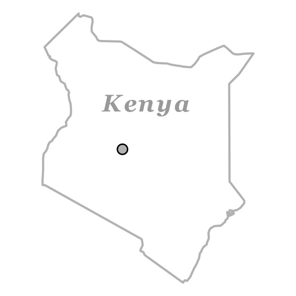
Plot Kenya outline
To provide a spatial reference, we’ll add the area location within Kenya as a map annotation. Therefore, we first load the outline of Kenya.
world <- ne_countries(scale = "medium", returnclass = "sf")
kenya <- world[ which(world$name_en == 'Kenya'), ]
Then, we create a plain plot of the outline and add the center point of the focus area as well as a label.
kenya_plt <- ggplot()+
  geom_sf(data=kenya, fill = 'white', color = rgb(0,0,0,.3),size=.5)+
  geom_point(data = bb_tib, aes(x = (x1+x2)/2,y = (y1+y2)/2),
             color = 'black',fill = rgb(0,0,0,.3), shape=21, size=2)+
  geom_text(data = tibble(x=37.8,y=2,lab='bolditalic(Kenya)'),aes(x,y,label=lab),
            size = 4, family = 'Georgia', parse = TRUE,color = rgb(0,0,0,.4)) +
  theme_void()+
  theme(legend.position = 'none',
        line = element_line(color=rgb(0,0,0,0), size = .1, linetype = 1, lineend = 'round'))
We turn this plot into a grob (grid object) to later use as annotation within ggplot().
kenya_grb <- kenya_plt %>% ggplotGrob()
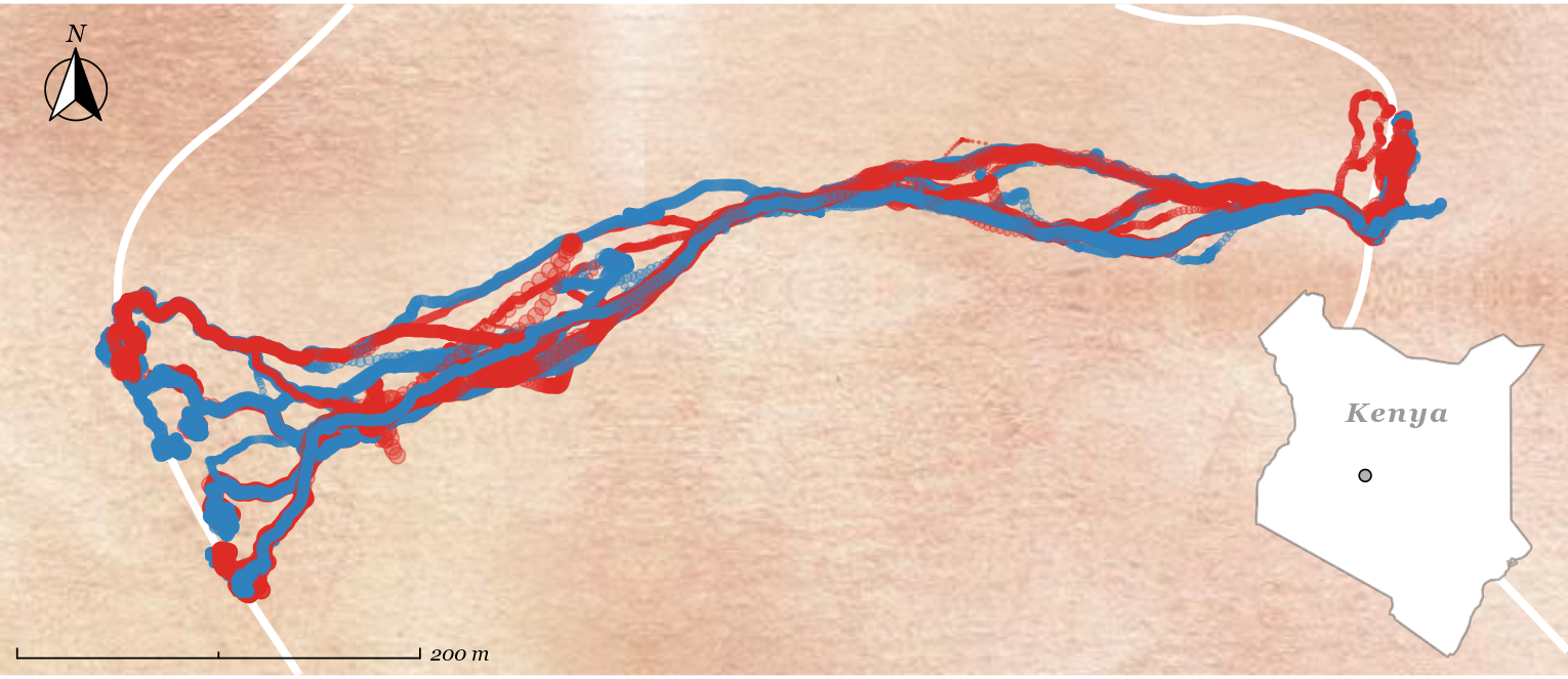
Generate base plot
Now, we can create the base plot that we’ll use for the animation.
p1 <- ggmap(stamen_map) +
  # add rivers
  geom_sf(inherit.aes = FALSE,
          data = smooth_rivers, size = 1.6, color = 'white')+
  # add movement data (bg lines) without timestamp - not animated
  geom_path(inherit.aes = FALSE, data = data_track %>% dplyr::select(-timestamp),
                       aes(x = long, y = lat, group = id),
                       color = rgb(0,0,0,.1),size=.2)+
  # add movement data (points) - this is the animated layer
  geom_point(inherit.aes = FALSE, data = data_track,
            aes(x = long, y = lat,
                color = sex, fill = sex,
                size = mass, group = id),
            shape = 21)+
  # add scale bar
  annotation_scale(location = "bl", width_hint = 0.3,height = unit(4,'pt'),
                   style = 'ticks', text_face = 'italic',text_family = 'Georgia') +
  # add compass
  annotation_north_arrow(location = "tl", which_north = "true",
                         pad_x = unit(10, "pt"), pad_y = unit(10, "pt"),
                        style = north_arrow_fancy_orienteering(text_face = 'italic',text_family = 'Georgia')) +
  # add the outline of Kenya
  annotation_custom(kenya_grb,xmin = 36.9275,xmax = 36.929,ymin = 0.35,ymax = 0.3518)+
  # adjust plot layout
  scale_y_continuous(expand = c(0,0))+
  scale_x_continuous(expand = c(0,0))+
  scale_fill_manual(values = alpha(clr, .3), guide=FALSE)+
  scale_color_manual(values = alpha(clr, .5), guide=FALSE)+
  scale_size(range = c(.2,3))+
  theme_void()+
  theme(legend.position = 'none',
        line = element_line(color=rgb(0,0,0,0), size = .1, linetype = 1, lineend = 'round'),
        plot.title = element_text(hjust = 0.5,face = 'italic',family = 'Georgia',margin = margin(t = 10, b = -20)))
Animate
Finally, all that is left to do is to chop the base plot apart according to the time points of the GPS positions and to stitch together the final gif file.
We first use the syntax of gganimate to define the timestamp column as the dimension along which the data will be animated.
anm <- p1 +
  ggtitle('{format(with_tz(frame_time, tz = "Etc/GMT-3"), "%H:%M:%S")}')+
  transition_time(timestamp) +
  ease_aes('linear')+
  exit_shrink()
Then, we render the animation and export the gif file.
animate(anm, nframes = 100, end_pause = 10)
anim_save('collective_movement.gif')
References
Crofoot, MC, RW Kays, and M Wikelski. 2015. “Data from: Shared Decision-Making Drives Collective Movement in Wild Baboons.” Movebank data repository. https://doi.org/doi:10.5441/001/1.kn0816jn.
Strandburg-Peshkin, Ariana, Damien R. Farine, Iain D. Couzin, and Margaret C. Crofoot. 2015. “Shared Decision-Making Drives Collective Movement in Wild Baboons.” Science 348 (6241). American Association for the Advancement of Science: 1358–61. https://doi.org/10.1126/science.aaa5099.
Uberti, Oliver, and James Cheshire. 2018. Where the Animals Go: Tracking Wildlife with Technology in 50 Maps and Graphics. S.l: Penguin Books Ltd.