genotype frequencies

Preparation:

To be able to plot genotytpe frequencies, we need a genotype table where genotypes are encoded as 0,1, & 2 (homozygous reference allele, heterozygous and homozygous alternative allele).

This can be easily generated from a vcf file using VCFtools:

vcftools \
  --gzvcf input.vcf.gz \
  --out  genotype_table \
  --012

Unfortunately the vcftools output has the wrong orientation (samples as rows, sites as columns). So before we reed the genotypes into R they are transformed using awk:

awk '
{
    for (i=1; i<=NF; i++)  {
        a[NR,i] = $i
    }
}
NF>p { p = NF }
END {
    for(j=1; j<=p; j++) {
        str=a[1,j]
        for(i=2; i<=NR; i++){
            str=str" "a[i,j];
        }
        print str
    }
}' genotype_table.012 | gzip > genotype_table.012.trans.txt.gz

R setup

To efficiently plot the genotypes frequencies we make use of the ggtern package as well as of the tidyverse (and of the hypogen package):

library(tidyverse)
library(ggtern)

Loading the data into R

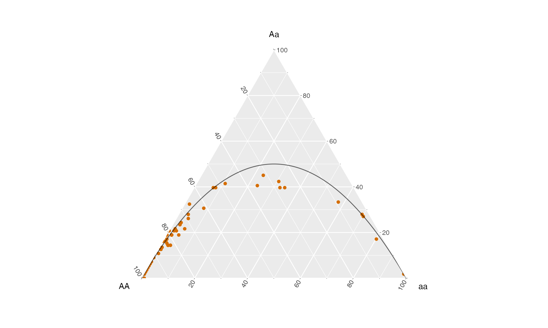
The package hypogen provides the function hypo_import_genotype_freq() which can read the transformed genotypee table and directly computes genotype frequencies:

file_genotypes <- system.file("extdata", "genotype_table.012.trans.txt.gz", package = "hypogen")

genotype_freqs <- hypo_import_genotype_freq(file_genotypes)

This table can be directly plotted using gggtern. As a reference we also make use of the hypogen function hypo_hwe() to indicate Hardy-Weinberg genotype frequencies:

ggplot() +
  coord_tern()+
  geom_point(data = genotype_freqs,
             aes(x = AA, y = Aa, z = aa ),
             col = hypo_clr_LGs[18]) +
  geom_path(data = hypo_hwe(n = 100),
            aes(x = AA, y = Aa, z = aa ),
            color ='black', alpha = .6)

---